In this post, we dive into V-JEPA, which stands for Video Joint-Embedding Predicting Architecture, a new collection of vision models by Meta AI. V-JEPA is another step in Meta AI’s implementation of Yann LeCun’s vision about a more human-like AI. Several months back, we’ve already covered Meta AI’s I-JEPA model, which is a JEPA model for images, and now we focus on V-JEPA, which is the JEPA model for videos, and as we’ll see in this post, there are many similarities between the two. If you’re new to the JEPA models, then don’t worry, no prior JEPA knowledge is needed to follow through. V-JEPA was introduced in a recent paper titled: “Revisiting Feature Prediction for Learning Visual Representations from Video”, and our focus here is to explain this paper, to understand what is the V-JEPA model about and how it works.
We’ll decipher the paper title meaning as we go, and our first step is to explain the second part of the title. What is the meaning of learning visual representations from video?
Before diving in, if you prefer a video format then check out the following video:
Video Visual Representations
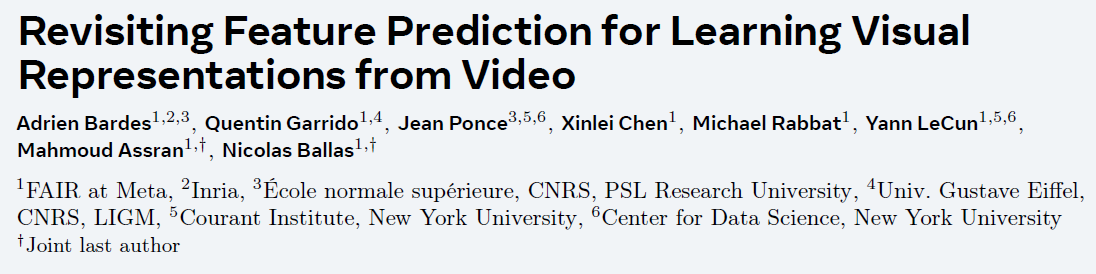
Say that we have multiple tasks that we want to solve, for example, given a video of a cat, we want to run it via an action classification model, to tell whether the cat is sleeping. And, say that we also want to run the video via a motion detection model to tell whether the cat is walking.
Without Visual Representations
One way of achieving both goals is to train two models, one dedicated specifically for action classification and the other dedicated specifically for motion classification, where each one is fed with the cat input video, and output the results for the specific task. This process can be complex and we might also need to use pretty large models depending on the task complexity. But there is a different way to approach this.
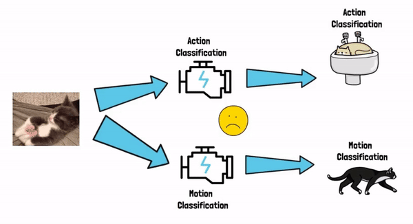
With Visual Representations
Starting with the end in mind, say that we’ve finished the training process of V-JEPA. We now have a model, call it V-JEPA encoder, that can yield visual representations from video. In simple words, the model can get the video as an input, and yield vectors of numbers, which are the visual representation of that video, these vectors are also referred as visual features or semantic embeddings. The visual representation captures the semantic of the input cat video, and once we have it we can feed that as an input to small and simple models, that target the specific tasks that we want to solve.
Feature Prediction
Now that we have an idea about the meaning of learning visual representations from video, let’s start to understand the meaning of the first part of the paper title. What is the meaning of feature prediction?
Feature Prediction with I-JEPA
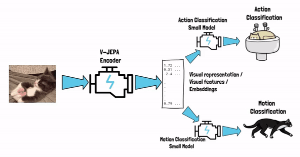
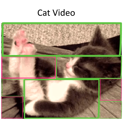
Let’s first remind to ourself the idea with I-JEPA. The concept is to predict missing information in abstract representation space. Given an image of a cat, we use part of the image as context, marked above with a green square, and using that context only, we predict information in other parts of the image, called targets, such as the cat leg and the cat ear, that are marked with pink rectangles. However, we do not predict the cat leg pixels themselves in this process, rather, we predict embeddings that capture the semantics of this cat leg. So we predict features, and not pixels.
Feature Prediction with V-JEPA
With V-JEPA the idea is similar, but with important nuances. Given a cat video, we take a few locations as targets, marked above with pink, and this time all of the other locations are used as the context, as we can see again in green, and we use that context to predict information in the targets. An important note here is that we use the same spatial area for the context and the targets across all of the video frames. So, one area of the video, across time, is used to predict other areas of the video across time. Doing it this way makes the task much harder to predict, since if we would use different areas for different video frames there would be an overlapping in the locations of the context and targets, just in different times, and the model could use the context it has on the target from a different frame, since usually the video does not change much in the same area in a short time.
The JEPA Framework

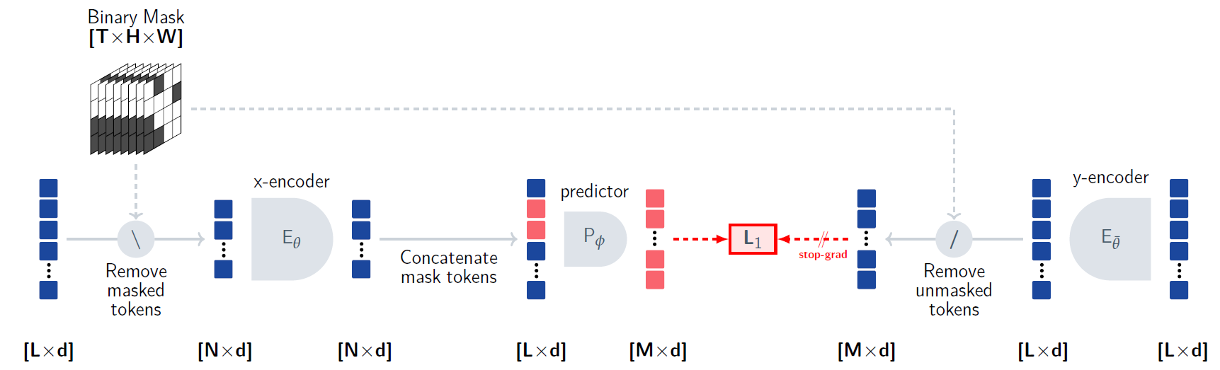
Now that we have the main idea in mind, let’s start to dive into the JEPA framework. Before diving into the specifics of V-JEPA, we first review the high-level components in JEPA using the above figure from the paper. We can see there are three main components here, the x-encoder, the predictor, and the y-encoder, and a loss function.
The x-encoder
The x-encoder is the main component which will be the outcome of the JEPA process. The x-encoder is in charge of encoding the input x. The inputs are the context blocks which we’ve just saw. The results from the encoder are passed to the predictor.
The Predictor
The predictor gets the output of the x-encoder in order to predict features, or in other words, in order to predict the representation of the information in the target blocks, such as the cat leg. And how the predictor knows which features to predict? This is based on the input z, which guides the predictor what to predict. In practice z provides the locations of the target blocks. Then, we see that the predictor output is compared with an output from the y-encoder. So, what is the y-encoder?
The y-encoder
The y-encoder gets the target blocks as input directly and yields representations for them.
JEPA Loss And Components Update
On one hand we have the predicted representations (x-encoder -> predictor), based on the context block, and on the other hand we have representations, calculated directly from the target blocks (y-encoder). The difference between them is used to calculate the loss. And using the gradients from that loss we train both the predictor and the x-encoder, but not the y-encoder. The y-encoder is updated using a moving average of the x-encoder weights. The reasoning behind that is to avoid model collapse, to avoid a situation where the encoders will learn for example to always yield zeros to minimize the loss. So, it is not updated using the loss, but because it is based on the moving average it is also not identical to the x-encoder.
I-JEPA Training Process
We are now ready to dive in with more details. First, we review the details for images with I-JEPA since it is a bit more intuitive to understand, and then we’ll see how it works for videos with V-JEPA. If you already have a good understanding of I-JEPA you may jump directly to the next section about V-JEPA Training Process.
I-JEPA has the same three components we mentioned earlier, a context encoder, mentioned as x-encoder before, a target encoder, mentioned as y-encoder before and a predictor. Each of them is a different vision transformer model.
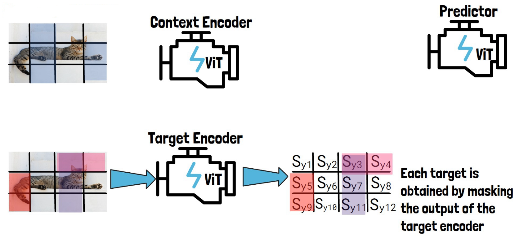
The Target Encoder
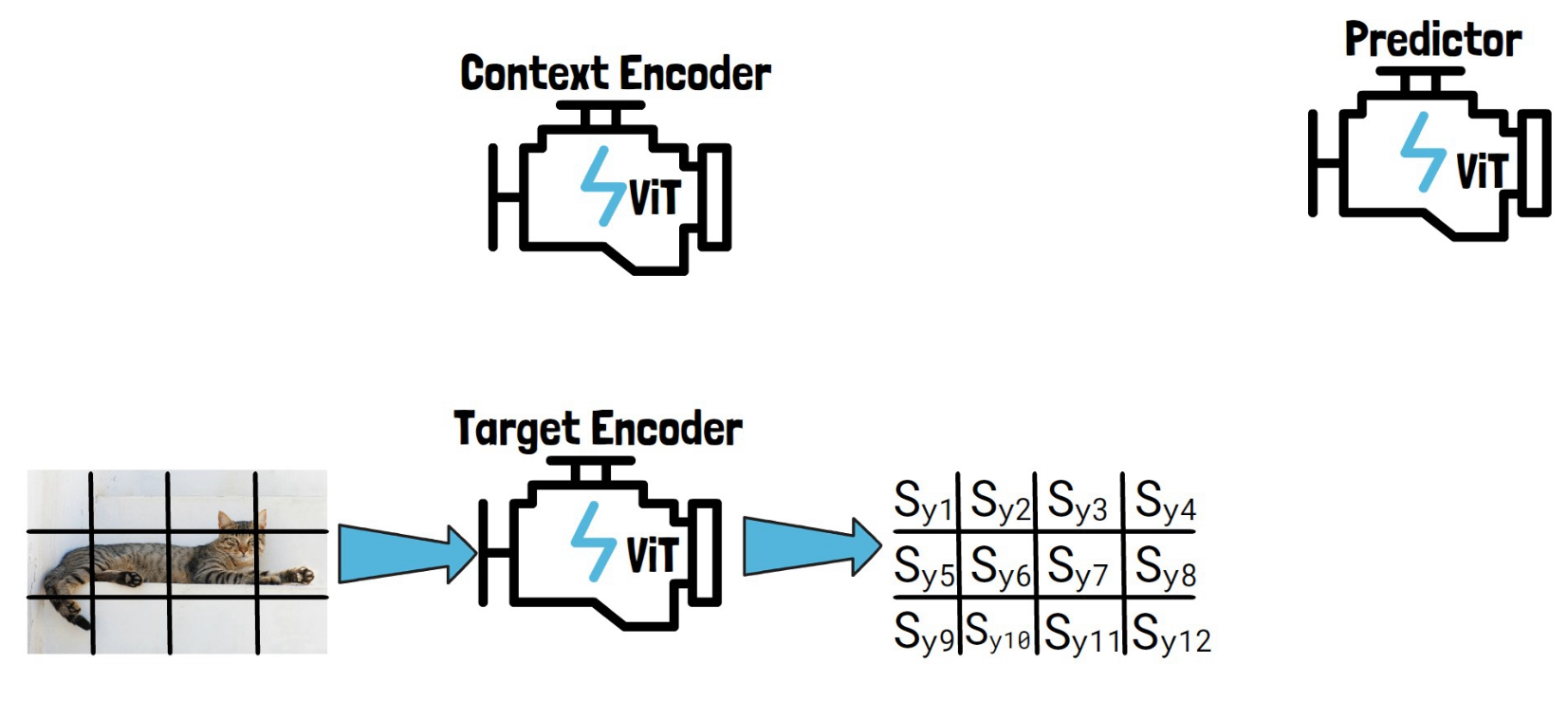
Given an input image like this image of a cat, we convert it into a sequence of non-overlapping patches (the black lines). We then feed the sequence of patches through the target encoder to obtain patch-level representations. We mark here each representation with Sy and the number of the patch, each Syi is the representation of the corresponding patch, created by the target encoder.
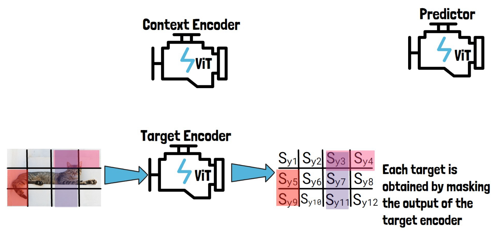
Then, we sample blocks of patch-level representations with possible overlapping, to create target blocks to predict and later calculate the loss on. In the example above we’ve sampled the following three blocks – (1) Sy3, Sy4 (2) Sy3, Sy7, Sy11 (3) Sy5, Sy9. On the left we see the corresponding patches on the image for reference, but remember that the targets are in the representation space as we have on the right. So, each target is obtained by masking the output of the target encoder.
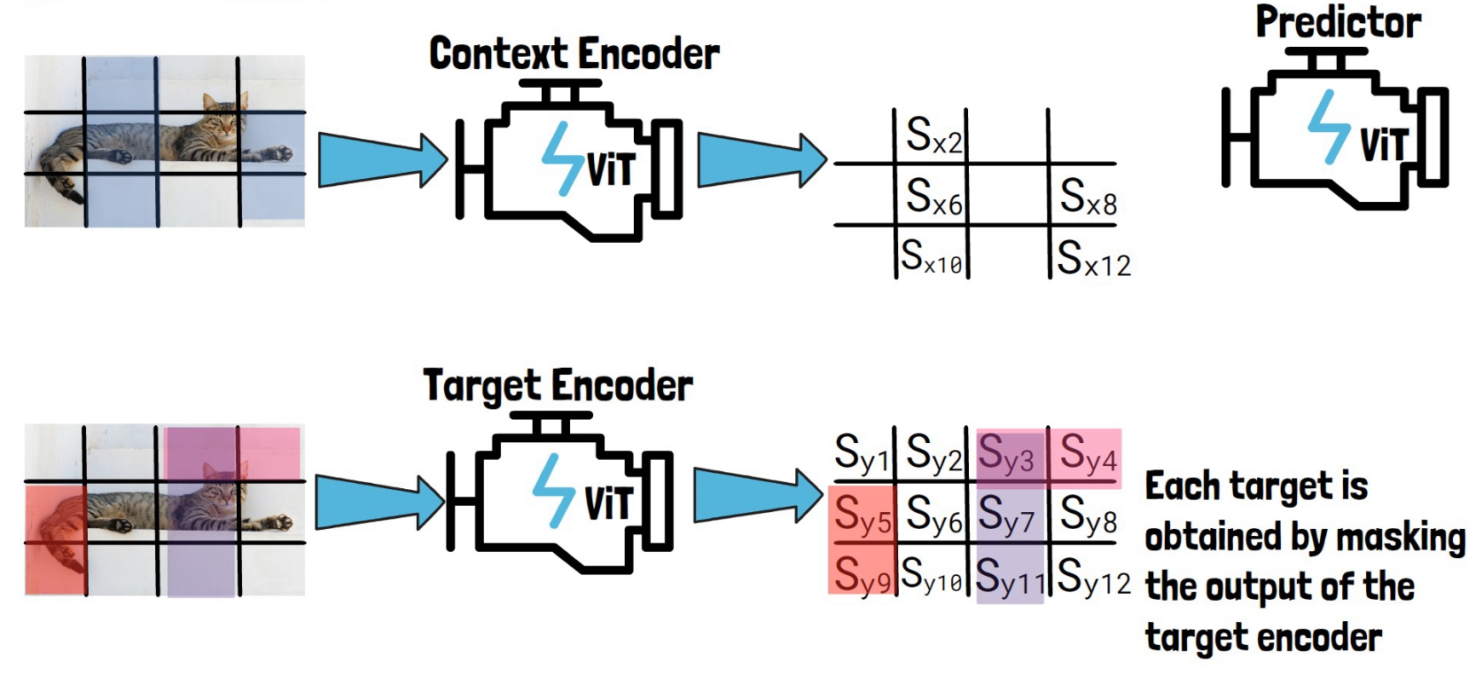
The Context Encoder
To create the context block, we take the input image divided into non-overlapping patches and we sample part of it as the context block, as we can see in the picture below to the left of the context encoder.
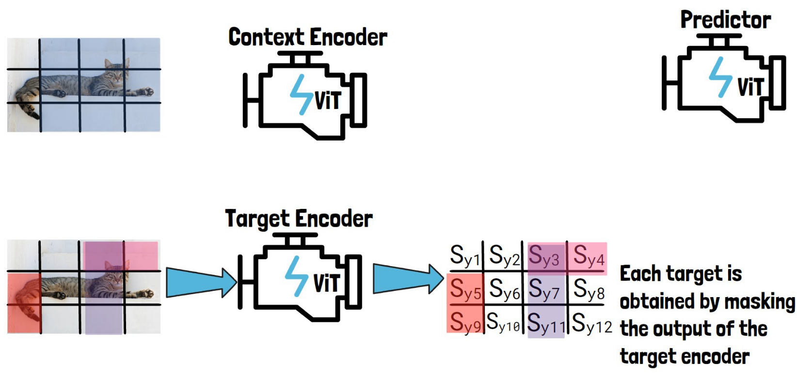
The sampled context block is by-design significantly larger in size than the target blocks, and also sampled independently from the target block, so there can be a significant overlap between the context block and the target blocks. So, to avoid trivial predictions, each overlapping patch is removed from the context block, so here out of the original sampled block we remove overlapping parts to remain with the following smaller context block as we see in the picture below on the left of the context encoder.
We then feed the context block via the context encoder to get patch-level representations for the context block which we mark here with Sx and the number of the patch, as we can see in the picture below.
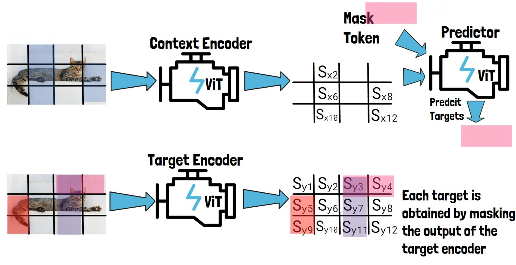
The Predictor
Now we want to use the predictor to predict our three target block representations. So, for each target block representation, we feed the predictor with Sx, the output from the context encoder and a mask token. The mask token includes learnable vector and positional embeddings that match the target block location. The predictor then predicts the representation of that target block. Following are three pictures, for each target block.
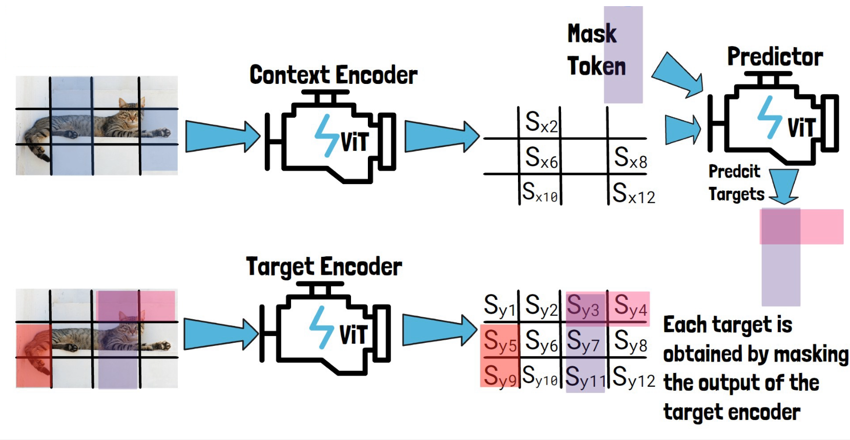
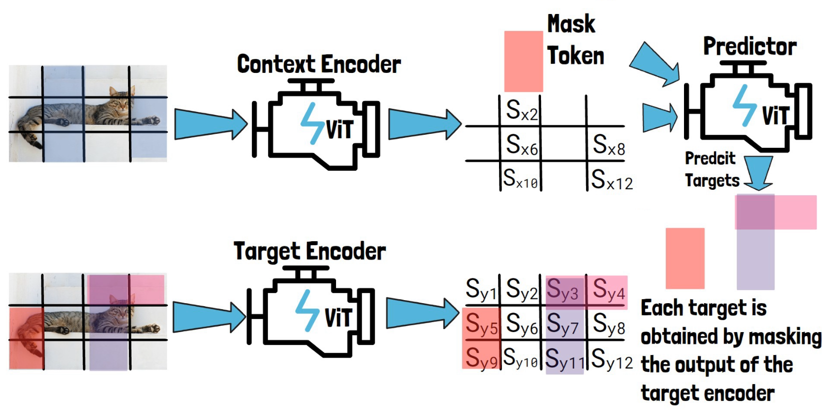
Finally, we get predictions of the target block representations from the predictor for each target block, and calculate the loss by the average L2 distance between the predictions, to the representations we got for the target blocks from the target encoder. The context encoder and the predictor learn from that loss, while the target encoder parameters are updated using a moving average of the context encoder parameters. Finally, at the end of the training process, our trained context encoder is capable of generating highly semantic representations for input images, and the researchers showed that using these representations they can achieve remarkable results in downstream tasks.
V-JEPA Training Process
Now that we understand how I-JEPA works, it should be easier to understand how V-JEPA works. To understand V-JEPA we will use the above figure from the paper.
Flatten the input to patches
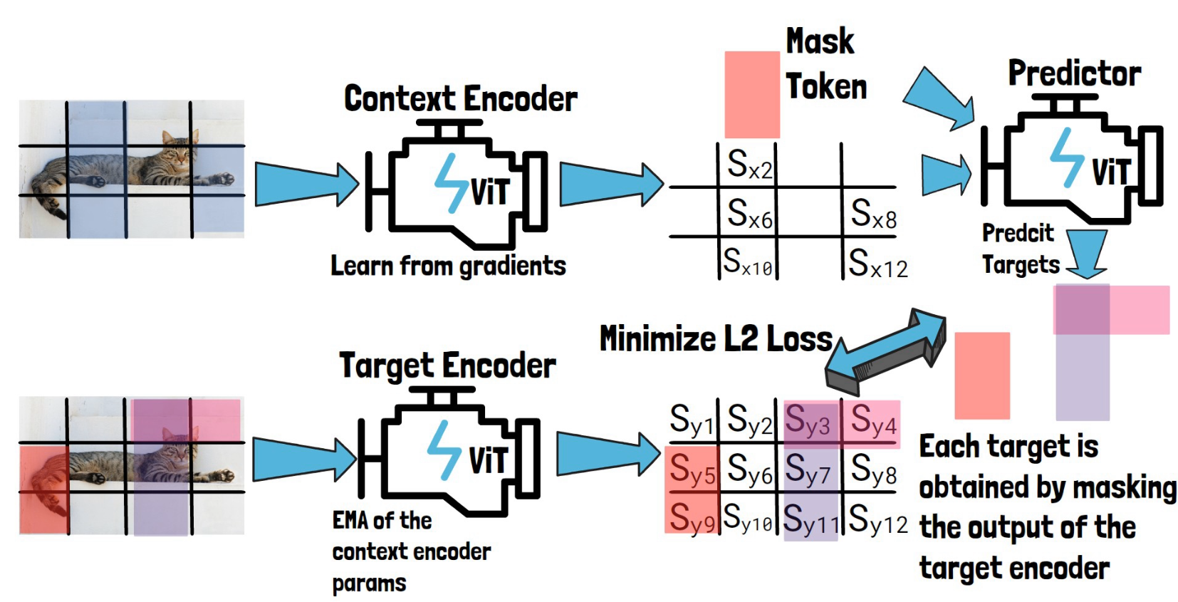
Our input is a video, and different than images, we now have an additional dimension which is the time dimension. We can see on the left an example for how it is modeled in the shape of the mask. The video is flattened to patches, so we can feed it into a vision transformer. The patches consist of a 16 X 16 pixels blocks spanning on two adjacent timeframes.
Dividing the video to context and targets
We determine the target blocks locations using a mask. Recall we mentioned earlier that the target blocks have the same spatial area across the video frames, and we can see that now when observing the mask on the left of the drawing, where we have the same grayed areas across all of the frames. And all of the non-grayed areas are used as the context.
Predict representations for target areas of the video
As with images, we want to run the context via the x-encoder, so we remove the masked tokens, which are the targets, from the input sequence. Then, the x-encoder can process the context tokens to yield representation for the context. We then add learnable mask tokens to the x-encoder output with positional information about the target blocks, similar to I-JEPA. Using the encoded context and the mask tokens, the predictor predicts representations for the target blocks. And we see that these predictions are used to calculate the loss similar to what we’ve seen earlier with I-JEPA, except that here we use L1 instead of L2.
Loss with direct encodings of the target blocks
The right side of the loss is created using the y-encoder, which first encodes the entire sequence, to include attention between all tokens. Afterwards, we keep only the target blocks tokens, which we compare with the predictions. Notice the stop-grad on the right side of the loss, which is because as before, the y-encoder is not updated using the loss but rather is a moving average of the x-encoder to avoid model collapse.
V-JEPA Results
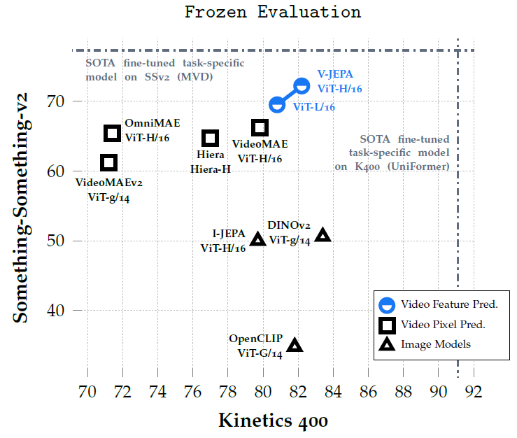
In the above chart from the paper, we can see the results of various strong models on two datasets, one is Something-Something-v2 on the y-axis, which measures motion-based tasks. The second dataset, on the x-axis, is Kinetics 400, which measures appearance-based tasks. We can see the results of the V-JEPA based models with blue, which outperforms other models on motion detection, including models that were trained on videos using pixel prediction methods. The results for appearance-based tasks are competitive, where DINOv2, which is trained on images performs best.
References & Links
- V-JEPA paper – https://ai.meta.com/research/publications/revisiting-feature-prediction-for-learning-visual-representations-from-video/
- V-JEPA code – https://github.com/facebookresearch/jepa
- V-JEPA video – https://youtu.be/4X_26j5Z43Y
- Join our newsletter to receive concise 1 minute read summaries of the papers we review – https://aipapersacademy.com/newsletter/
All credit for the research goes to the researchers who wrote the paper we covered in this post.