I-JEPA – A Human-Like Computer Vision Model

I-JEPA, Image-based Joint-Embedding Predictive Architecture, is an open-source computer vision model from Meta AI, and the first AI model based on Yann LeCun’s vision for a more human-like AI, which he presented last year in a 62 pages paper titled “A Path Towards Autonomous Machine Intelligence”.
In this post we’ll dive into the research paper that introduced I-JEPA model, titled: “Self-Supervised Learning from Images with a Joint-Embedding Predictive Architecture”. No prior knowledge of Yann LeCun’s vision is needed in order to follow along. We’ll explore what is more human-like in this model and dive deep into how it works.

If you prefer a video format, the a large portion of what we will cover is explained here:

Self-Supervised Learning For Images

Let’s start with an essential background about self-supervised learning in computer vision. So first, what is self-supervised learning? In short, it means our training data has no labels and the model learn solely from the images, which helps to capture common-sense knowledge from the data itself, which is important for learning in a more human-like method.
There are two common approaches for self-supervised learning from images, invariance-based and generative. We now review these common methods and then we’ll introduce the new I-JEPA method.

Invariance-Based Self-Supervised Learning

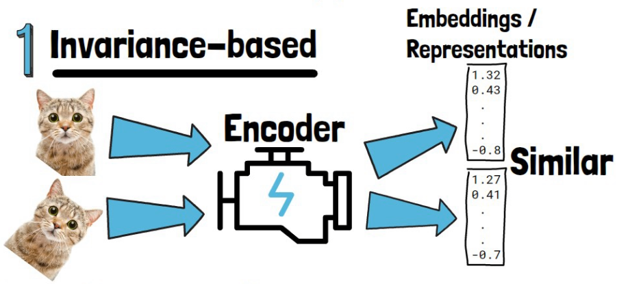
In the invariance based approach, we train an encoder to receive an image as input such as the cat images above, and produce vectors of numbers that represent the semantics of the image. These vectors are called embeddings or representations. The idea here is that during training we feed the model with similar images, such as the cat and the rotated cat images in the picture, and we optimize the encoder so it will yield similar embeddings to both images, because they have similar semantic meaning. Embeddings of not compatible images are trained to be dissimilar.
The different views of the same image are usually created using hand-crafted data augmentation techniques, such as geometric transformations, coloring and more.
This approach proved to reach high semantic levels. However, previous research has shown it comes with biases. Additionally, this technique is specific to images, meaning that if we would like to train other types of data it is not clear how to generalize this approach.
Finally, crafting proper data augmentation usually requires some level of prior knowledge about the data.

Generative Self-Supervised Learning

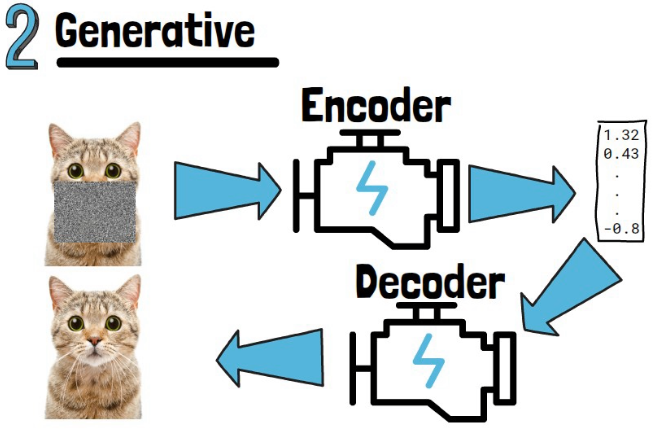
In this approach we also want to have an encoder that can get an image and generate meaningful embeddings. To train that encoder, during training we mask or corrupt random parts of the input image, and then use another model which is called a decoder, to get the embeddings the encoder returns, in order to reconstruct the image.
This approach can generalize well to other types of data, for example large language models (LLMs) are pretrained to predict the next word, or masked words.
Additionally, less prior knowledge is needed since there is no requirement to provide in advance images that are similar to each other.
However, this approach usually reaches lower semantic levels and underperforms comparing to the invariance-based approach.

I-JEPA Self-Supervised Learning

We are now ready to dive into the self-supervised learning approach that I-JEPA brings. We’ll dive into the architecture in details in a minute, but first let’s understand the goal and main idea. The goal is to improve the semantic level of the representations, but without using prior knowledge such as similar images created using data augmentation. The main idea in order to achieve that is to predict missing information in abstract representation space.

Let’s break this down step by step. Predict missing information is different than what we saw in the generative approach where the model is trained to reconstruct a noisy part. The meaning here is that given an input image like the cat image above, they use part of the image as context, marked here with the green square, and they use this context to predict the information in other parts of the image, like the ones marked with pink squares here.
So, we covered what missing information means, but what does it mean to predict in abstract representation space?
Let’s look at target 2 square for example, the model learns to predict that there is a cat leg in this block, but it doesn’t learn to predict the pixels of that leg. In generative approach, a model would learn to predict the explicit pixels to describe the cat leg, but in I-JEPA the model learns to predict embeddings that grasp the semantics of this cat leg.
We’ll see this in more details in a moment, but the idea is that the model is guessing that there is a leg here. This is more similar to how humans would guess missing parts of a picture rather than predicting the pixels. And this is also less prone to errors due to insignificant details since the model is focused on higher level semantics and not on the pixels.

I-JEPA Architecture and Training

Alright we’re now ready to explore how I-JEPA is built with more details.
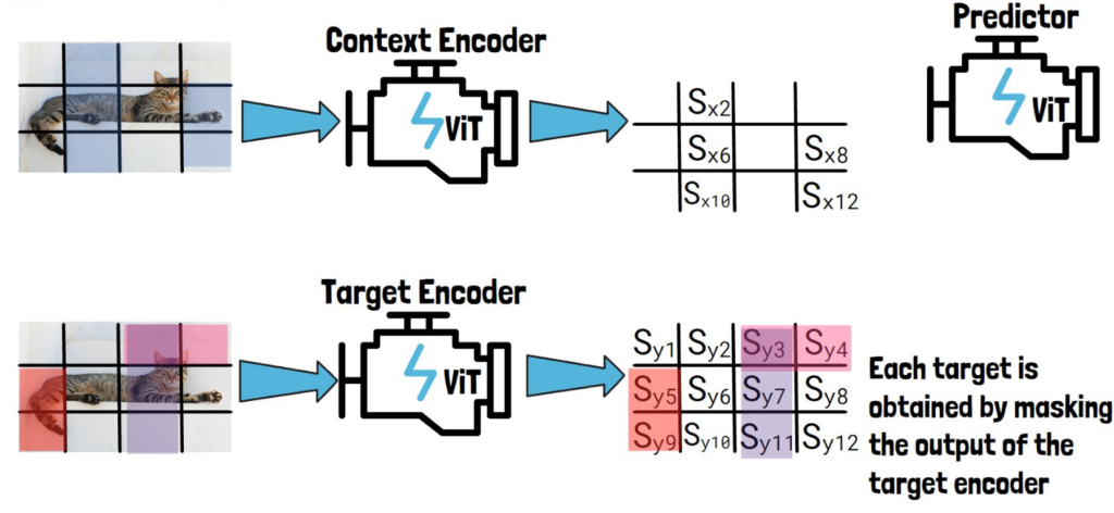
I-JEPA has three components, a context encoder, a target encoder and a predictor. Each of them is a different Visual Transformer model.
We now cover each of the three components to gain full understanding of I-JEPA architecture.

The Target Encoder

Given an input image like this image of a cat, we convert it into a sequence of non-overlapping patches (the black lines). We then feed the sequence of patches through the target encoder to obtain patch-level representations. We mark here each representation with Sy and the number of the patch, each Syi is the representation of the corresponding patch, created by the target encoder.

Then, we sample blocks of patch-level representations with possible overlapping, to create target blocks to predict and later calculate the loss on. In the example above we’ve sampled the following three blocks – (1) Sy3, Sy4 (2) Sy3, Sy7, Sy11 (3) Sy5, Sy9.
On the left we see the corresponding patches on the image for reference, but remember that the targets are in the representation space as we have on the right. So, each target is obtained by masking the output of the target encoder.

The Context Encoder

To create the context block, we take the input image divided into non-overlapping patches and we sample part of it as the context block, as we can see in the picture below to the left of the context encoder.

The sampled context block is by-design significantly larger in size than the target blocks, and also sampled independently from the target block, so there can be a significant overlap between the context block and the target blocks
So, to avoid trivial predictions, each overlapping patch is removed from the context block, so here out of the original sampled block we remove overlapping parts to remain with the following smaller context block as we see in the picture below on the left of the context encoder.

Below is a picture from the paper showing different examples of context and target blocks, where we can see that the context is larger but then reduced after removing overlapping patches. An important note here is that the size of the context and target blocks should be large enough in order to have a semantic meaning, which the model can then learn.

Going back to the architecture overview, we then feed the context block via the context encoder to get patch-level representations for the context block which we mark here with Sx and the number of the patch, as we can see in the picture below.

The Predictor

Now we want to use the predictor to predict our three target block representations.
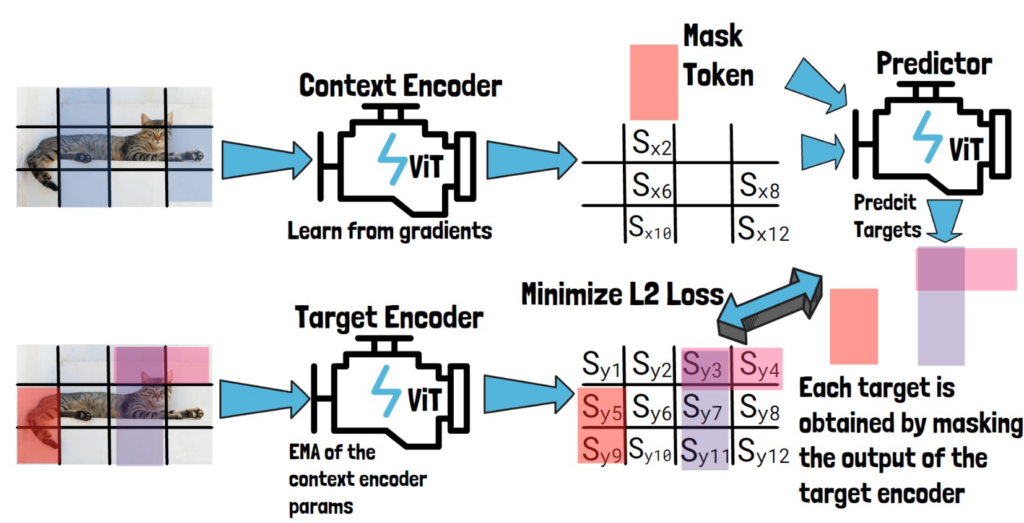
So, for each target block representation, we feed the predictor with Sx, the output from the context encoder and a mask token. The mask token includes learnable vector and positional embeddings that match the target block location. The predictor then predicts the representation of that target block.
Following are three pictures, for each target block.

Finally, we get predictions of the target block representations from the predictor for each target block, and calculate the loss by the average L2 distance between the predictions, to the representations we got for the target blocks from the target encoder.
The context encoder and the predictor learn from that loss, while the target encoder parameters are updated using exponential moving average of the context encoder parameters.
Finally, at the end of the training process, our trained context encoder is capable of generating highly semantic representations for input images, and the researchers showed that using these representations they can achieve remarkable results in downstream tasks.

References

• Paper – https://arxiv.org/abs/2301.08243
• Code – https://github.com/facebookresearch/ijepa
• Video – https://youtu.be/6bJIkfi8H-E

A recommended read for another fascinating advancement we recently covered that improves over the known mixture of experts can be found here – https://aipapersacademy.com/from-sparse-to-soft-mixture-of-experts/