In this post, we dive into a new research paper, titled: “Fast Inference of Mixture-of-Experts Language Models with Offloading”.

Motivation
LLMs Are Getting Larger
In recent years, large language models are in charge of remarkable advances in AI, with models such as GPT-3 and 4 which are closed source and with open source models such as LLaMA 1 and 2, and more. However, as we move forward, these models are getting larger and larger and it becomes important to find ways to improve the efficiency of running large language models.
Mixture of Experts Improves LLMs Efficiency
One development that has been adapted with impressive success is called Mixture of Experts (MoE), where the idea is that different parts of the model, which are the experts, learn to handle certain types of inputs, and the model learns when to use each expert. For a given input, a small portion of all experts is used, which makes this model more compute-efficient. One of the best open source models out there these days is a MoE model by Mistral, which is called Mixtral-8x7B.
Mixture of Experts on Limited Memory Hardware
While being compute-efficient, the MoE models architecture has a large memory footprint since we need to load all of the experts into memory. In the paper we review in this post, the researchers introduce a method to efficiently run MoE models with limited available memory using offloading, which even allows running Mixtral-8x7B on the free tier of Google Colab, which makes it much more accessible to researchers without a substantial amount of resources.
Before diving in, if you prefer a video format then check out the following video:
Mixture of Experts
Let’s start with a quick recap for how the mixture of experts method works. The common methods up until now are called sparse mixture of experts, and we also reviewed Google’s soft mixture of experts in the past. The idea with mixture of experts is that instead of having one large model that handles all of the input space, we divide the problem such that different inputs are handled by different segments of the model. These different model segments are called experts. What does it mean?
Mixture of Experts High-Level Architecture

In high level, we have a router component and an experts component, where the experts component is comprised of multiple distinct experts, each with its own weights. And given input tokens such as the 8 tokens here, each token passes via the router, and the router decides which expert should handle this token, and routes the token to be processed by that expert. More commonly the router chooses more than one expert for each token, so in the above example we choose 2 experts out of 4. Then, the chosen experts yield outputs which we combine together. These experts can be smaller than if we would use one large model to process all tokens, and they can run in parallel, so this is why the computational cost is reduced.
Input Encoding vs Tokens Generation
This above flow is repeated for each input token, so the second token also passes via the router, and the router can choose different experts to activate. For the input prompt, the tokens are handled together and we do not do this one after the other. However, for the generated tokens in the response, we have to go through this process token by token. This is an important distinction for the MoE offloading method we will explain in a minute. In this example we present a single layer, while there are usually more than one, so the outputs of this layer are chained to the next layer in the model.
MoE Offloading

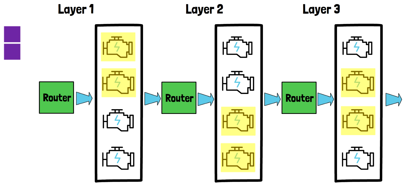
Let’s now add more layers to the model and discuss how offloading can help to improve the inference efficiency when there is limited memory. In the above image for example we have 3 layers, each layer has a router and 4 experts and each layer has its own weights. Note that this drawing is simplified in order to explain the offloading part.
Offloading Includes Only The Experts Weights
In a limited memory hardware, we cannot load the entire model into GPU memory. The experts weights are in charge for the majority of the model size. We can keep the other parts of the model constant in the GPU such as the routers, and self-attention blocks which are excluded from this drawing. And we’re now going to see how the experts weights can be loaded efficiently.
Phase 1 – Input Prompt Encoding

The generative inference consists of two phases. The first phase is input prompt encoding. Here simple offloading technique already works quite well. What does it mean? When we process the input prompt, we first load the experts of layer 1 into memory. We color them with yellow to represent they are loaded into the GPU memory. Then we feed the entire sequence to the first layer which handles all tokens in parallel.

Once finished, layer 1 experts can be unloaded and make room for the experts of the second layer. Similarly, when layer 2 is done processing, the experts of layer 2 can be unloaded to make room for the experts of layer 3. In real models in the wild we have more than 3 layers and this process could continue. If the GPU memory can hold the experts of two layers simultaneously then there is room for even more optimization since we could load the next layer experts during the processing of its preceding layer. But anyway, each layer experts are loaded only once, since we process the input sequence in parallel and layer by layer.
Phase 2 – Tokens Generation
In the second phase of the generative inference process it gets more interesting. The tokens generation phase is not only done layer by layer, rather in this case we also generate the tokens token by token and layer by layer. So acting the same results in loading and unloading all experts for each generated token. So here the researchers suggest to include a LRU cache. How does it work?
Experts LRU Cache

When generating the first token, we start with the first layer. In the example above the activated experts are the first and the third experts. So only these experts are loaded, and are kept in memory for now. Then similarly for layer 2 we load the activated experts only, in the example above these are the first and last experts. An important point to understand here is that if we want to only load the activated experts, we have to wait for the results of the first layer, since choosing the activated experts by the router is based on the previous layer output. Once we have the output of the second layer, we do the same in the last layer, in the above example the activated experts are the middle ones.
Now, when we start the process to generate the second token, we already have 2 experts loaded in the first layer. Say for example that the activated experts in the first layer for the second token are the top two, then we only need to load the second expert, so we saved time here. Similarly, if in the second layer the activated experts are now the last two, then we only need to load the third expert. And in the last layer let’s assume for example that the activated experts are the same, in this case there is no need to load any expert. In this example the LRU cache size is 2 for all layers. The researchers have found that the LRU cache hit rate is large, meaning there are many cases where the activated expert is already loaded when we need it, so it improves the efficiency of the inference process.
Experts LRU Cache Paper Example
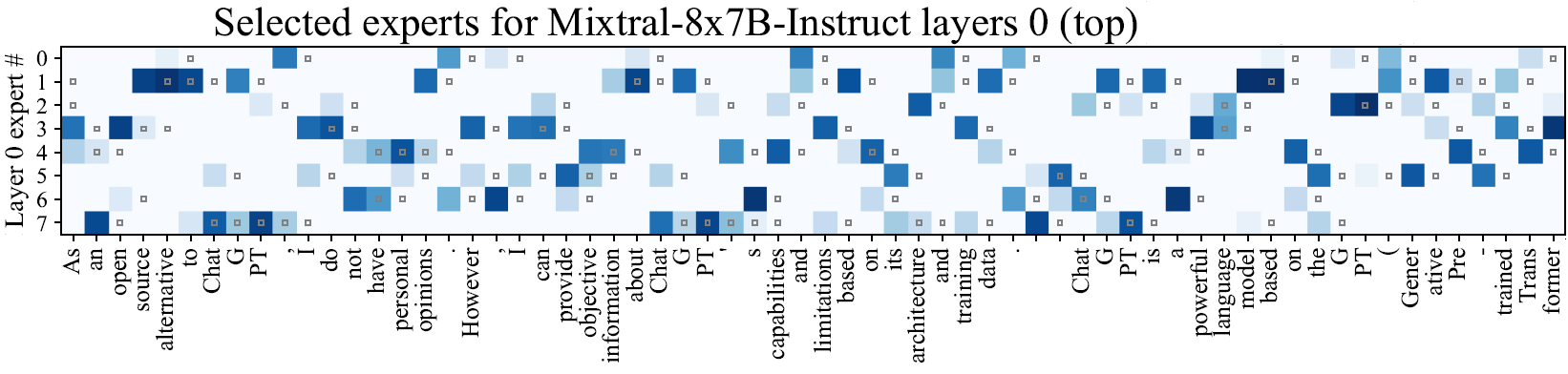
In the above figure from the paper, we can see an example for the LRU cache in action. We see here the experts of layer zero where each row represents a different expert in that later. The columns, as we can see at the bottom, represent a sequence of tokens. The blue cells, such as experts 3 and 4 in the first column, represent that these experts were active while encoding the token, where deeper blue means that the router provided a higher value for that expert. The small gray squares represent the experts that are saved in the LRU cache. Looking at the second column, we see that the experts we have in the LRU cache are experts 3 and 4, since they were the ones which were activated for the previous token. In this case one of them, expert 4 is used also for the second token, while we need to replace expert number 3. Looking at the rest of the tokens, we can see there are many cache hits (gray square in a blue cell), where we re-use an already loaded expert. But we can also see that there are quite a lot of cache misses (blue cells without a gray square), where we still need to wait and load an expert that is not in the cache.
Speculative Experts Loading

While the LRU cache helps, the researchers have found another method to accelerate the model, which is speculative experts loading. To explain this method, let’s review the example above, when we proceed to generate the third token in the drawing we saw earlier. In the first two layers, there is no change from before and we still use the LRU cache as we did. For simplicity let’s assume in this case there was no change in the loaded experts. With the third layer we reach the interesting part. We already have two experts loaded in the LRU cache. However, another step that is added is that while we had the results from the first layer, we can try to guess based on them which experts will be used in the third layer rather than waiting for the results from layer 2. We do that without introducing any new component, but rather by feeding the results from layer 1 to the router of layer 3. Then, if the guess is that the activated experts will be the first two experts, then we do the change in the loaded experts, in this case loading the first expert. And we do that in parallel while layer 2 is still running. When we have the results of layer 2, we still pass them via the router, and if the guess was wrong then we fix and load the real activated experts.
How Well Does It Work?

In the following figure from the paper, evaluated using Mixtral-8x7B on the OpenAssistant dataset, we can see on the left the hit rate for the LRU cache, and for example when the cache is of size 2 (the orange line), we can see that we have the correct expert in the cache in about 40% of the times, and if we increase the cache size to 4, if the hardware we use has enough memory for this, then the hit rate jumps to approximately 60% or more. On the right chart, we can see the improvement when using speculative loading. In the regular lines that are not dashed, we can see in blue, the if we prefetch the experts of one layer ahead based on the speculative loading guess, then we have the correct expert loaded for about 80% of the times or a bit more. And with fetching 3 experts it improves to over 90%. The dashed and dotted lines show the result when looking more than one layer ahead, which shows that the prediction of which experts are active is less accurate as we look further ahead.
Mixed MoE Quantization
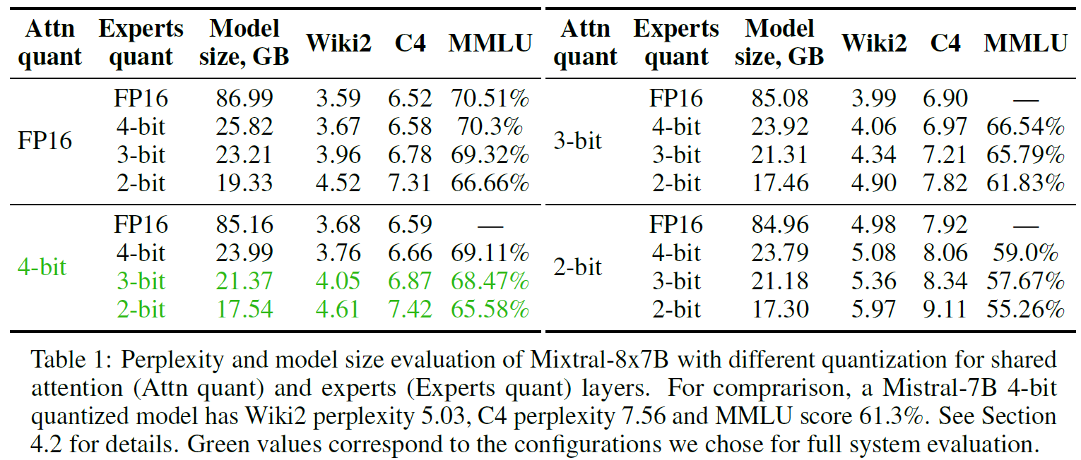
The researchers have tried to find a setting for the model that will be the most beneficial tradeoff between model size and performance for offloading. In the above table from the paper, we can see the researchers have tried four different quantization methods for the attention layers and for the experts, and evaluated them using the perplexity of Wiki2 and C4, and MMLU accuracy. In green we can see two chosen settings, both with 4-bit quantization for the attention layers and one with 3-bit and the other with 2-bit quantization for the experts. We can see that in the chosen settings the model size is relatively smaller comparing to other versions but still provides relatively good results.
Inference Speed

Finally, we can see the inference speed when using the offloading methods described in the paper. In the following table we can see the results on low-tier GPUs for the two chosen model settings where each value represents the number of tokens generated per second. When using the full algorithm, we can see that with 2-bit experts we reach inference speed between 2 to 3 tokens per second. We can see in the bottom row the results for using naive offloading where we just load the entire layer experts when needed, which is significantly slower. Specifically for Google Colab we see the inference speed is 2 tokens per second with the paper method comparing to 0.6 without it.
Links & References
- Paper – https://arxiv.org/abs/2312.17238
- Video – https://youtu.be/OSV243XPoKY
- Code – https://github.com/dvmazur/mixtral-offloading
- Join our newsletter to receive concise 1 minute read summaries of the papers we review – https://aipapersacademy.com/newsletter/
All credit for the research goes to the researchers who wrote the paper we covered in this post.