In this post, we dive into H-JEPA (Hierarchical Joint Embedding Predictive Architecture) an hierarchical world model co-authored by Yann LeCun that lets world model based AI agents plan long-horizon tasks.
Yann LeCun’s World Models and JEPA: Why AI Agents Need to Imagine
LeCun’s Vision: World Models for Human-Like AI
Yann LeCun has long argued that more capable human-like AI needs a world model, one that understands how the world behaves, so an agent can imagine the consequences of its actions before taking them. Since leaving Meta to start AMI Labs, LeCun and his collaborators have continued pursuing this vision.
What Is JEPA (Joint Embedding Predictive Architecture)?
LeCun’s proposed architecture is JEPA, short for Joint Embedding Predictive Architecture. Its main idea is to predict the future in abstract representations rather than raw pixels.
We covered LeWorldModel, a recent JEPA based world model in a previous post, but you don’t need it to follow along.
How Can a World Model Help an Agent Plan?
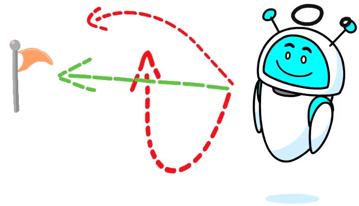
So how can a world model help an agent plan? Given a goal, the agent can imagine how different sequences of actions might play out, then choose the actions expected to move it closer to its goal.
However, long-horizon planning is what real tasks demand, and current JEPA world models still struggle to plan far ahead.
Why Long-Horizon Planning Is Hard for JEPA World Models
- One reason is that many of them plan at a single timescale. To predict far into the future, they have to chain together many small steps. As the planning horizon grows, prediction errors can compound, and the number of possible action sequences to search increases.
- Moreover, a single latent representation has to serve two different purposes: capturing the details needed for precise, low-level control while also representing progress toward a high-level goal.
What Is H-JEPA?
This is where a new paper co-authored by LeCun comes in, titled H-JEPA: End-To-End Learning Of Hierarchical World Models For Visual Planning.
The Core Idea: A Hierarchy of World Model Components at Different Timescales
We can understand the intuition from the following figure from the paper.
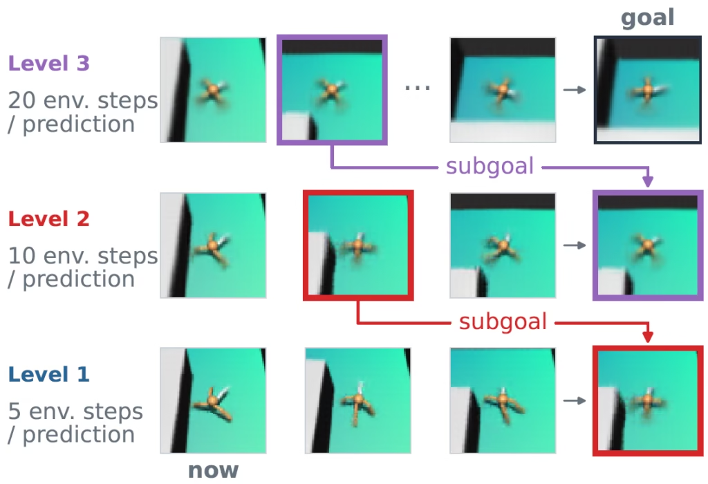
On the left, we see the key idea of organizing the world model into a hierarchy of components, each operating at a different timescale and learning its own representation. Here we have three levels but in general there could be more.
How Hierarchical Planning Works
Planning works from coarse to fine.
- Highest level: The highest level comes up with a high-level plan. Basically, to reach its end goal, the agent imagines where it should be 20 steps from now in each prediction step. Its plan becomes the sub goals of the level below it. Its first prediction step of where it should be 20 steps from now becomes the subgoal of the intermediate level.
- Intermediate level: The intermediate level then predicts two steps to reach that 20 step goal. Its first prediction step shows where it should land on 10 steps from now, which becomes the subgoal of the lowest level.
- Lowest level: Finally, the lowest level produces the concrete actions the agent takes.
How H-JEPA Is Trained: Hierarchical Representation Learning
So how exactly is this hierarchy trained, and how does the planning process work? Let’s start with a high-level overview of the training process, and then gradually add more details.
For simplicity, let’s first understand the lowest level, which acts as a standard JEPA world model. This is the building block of H-JEPA, similar to the one we saw in LeWorldModel. We’ll then build higher levels on top of it. In practice, though, all levels are trained together, end-to-end.
Level 1: Training the Base JEPA World Model
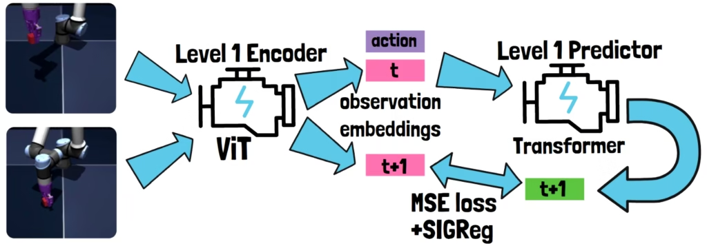
To learn how the world behaves, the model is trained on sequences of observations and the actions performed between them. For example, on the left. we have two consecutive observations of a robotic arm. The action between them could be moving the arm in a certain direction.
The idea is to use the earlier observation and the action to predict what comes next, which is the second observation. But JEPA doesn’t predict future pixels. Instead, it predicts the future in a semantic representation space. This happens in two stages using an encoder and a predictor components.
The Encoder and Predictor: Predicting in Semantic Representation Space
- First, each observation is converted into a semantic representation by an encoder, which is modeled as a Vision Transformer (ViT). The result of the encoder for each image is a single vector capturing the high-level content of the image.
- Then, another component called the predictor, modeled as a Transformer, receives the representation of the current observation, along with an embedding of the action, and predicts the representation of the next observation.
Training Loss: MSE Prediction Loss and SIGReg to Prevent Representation Collapse
During training, this prediction is compared with the representation produced by the encoder for the actual next observation. The model is optimized to make these representations match using an MSE loss. A regularizer called SIGReg is applied as well to prevent representation collapse. We explain the regularizer and the training process in more depth in the LeWorldModel breakdown.
This gives us the first level of the hierarchy. Now let’s see how we can add a second level on top of it.
Level 2: Adding a Second Level on Top of the JEPA World Model
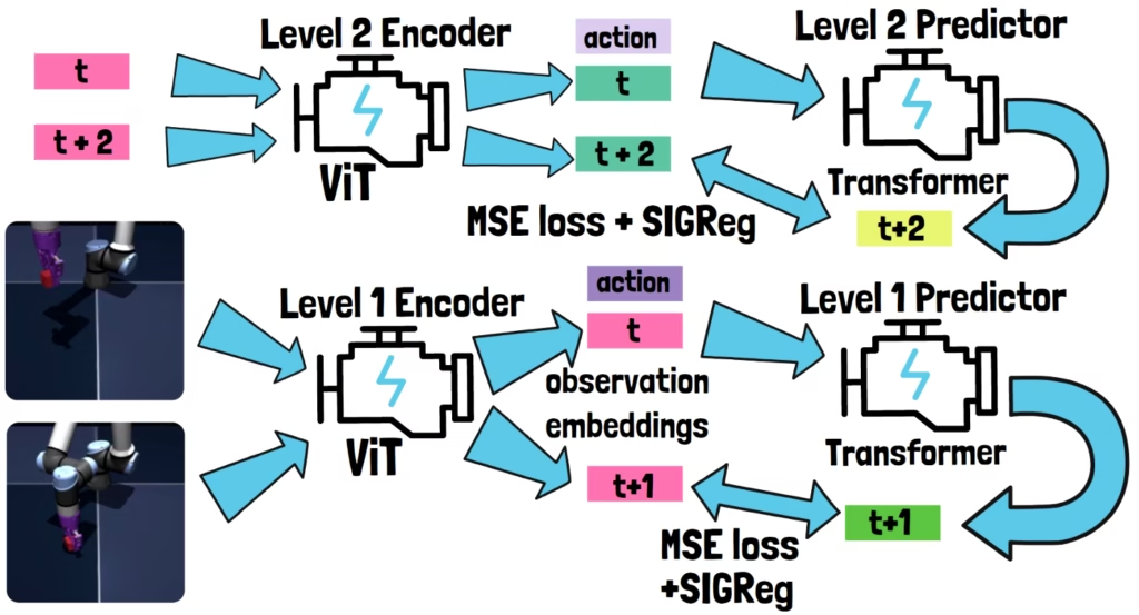
Level 2 State and Prediction Target: Predicting Further into the Future
The second level doesn’t work directly with images. Instead, its current state is the embedding produced by the first level for the current observation. The second level should behave similarly during training, meaning that given the current state and an action, it should predict the state in its own abstract representation space.
But what exactly is the next state here?
We don’t want the second level to predict every consecutive state from the first level. Instead, we want it to predict further into the future. So it is not the embedding of the next observation from the previous layer. Instead, it is the one that comes another step after that. This means it takes every second representation from the first level, and predicts the representation two lower-level steps into the future.
The choice of looking two steps ahead is a hyperparameter of the model.
Level 2 Encoder and Predictor: Learning a Separate Representation Space
- The second level has its own encoder, so it learns its own representation space. Both the current and future lower-level representations are passed through the second level’s own encoder to generate embeddings in the second layer representation space.
- The second layer also has its own predictor, also a Transformer, that should use the current embedding and an action to predict its own next observation.
Higher-Level Actions: Combining Low-Level Actions with an Action Encoder
So, what action do we use in the second layer? The actions also come from the lower level, but since we skipped a step from the first level, there are now two lower-level actions between the current state and the future state.
These two actions are combined by an action encoder into a single higher-level action embedding. We’ll leave the action encoder out of the drawing for simplicity, but it is also trained as part of the process.
Level 2 Prediction and Loss
The second-level predictor receives the current higher-level representation and action embedding, and predicts its next representation.
Just like before, the prediction is compared with the representation of the actual future state, using the same prediction loss and regularization.
Adding More Levels: End-to-End Training of the Full H-JEPA Hierarchy
From here we could add a third layer that uses the embeddings from the second layer, and so on. Importantly, all levels are trained together end-to-end. Gradients from the higher levels flow back into the first level’s encoder.
How H-JEPA Plans: Hierarchical Planning with Gradient Descent
Let’s now move on to see how H-JEPA can be used to plan a sequence of actions.
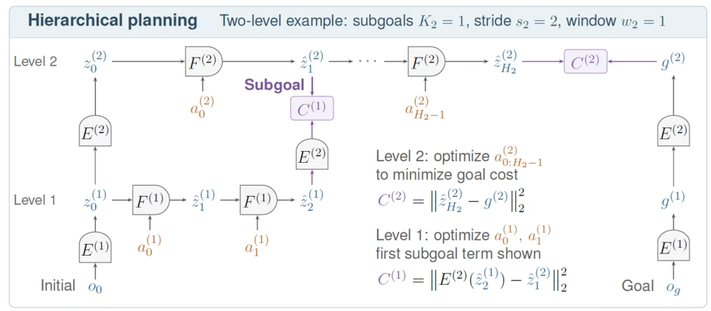
Let’s understand the planning process using the following figure from the paper. For simplicity, it shows a hierarchy with just two levels.
Planning Inputs: Current Observation and Goal Observation
We start with two image observations: the current observation and the goal observation.
- On the bottom left, we have the initial observation, where planning starts. It is passed through the encoders of both levels, giving us the current state representation at each level.
- On the bottom right, we have the goal observation, which is also passed through both encoders, giving us the goal representation at each level.
High-Level Planning: Optimizing Action Sequences in Representation Space
Now, planning starts from the top.
The second level needs to find a sequence of high-level actions that takes it from the current state to the goal state, in its own representation space.
- It starts with an initial guess for these actions. Then, the second level predictor imagines where they would lead, until we get a final predicted state.
- We measure the distance between this final prediction and the goal representation. Since the entire process is differentiable, we can use gradient descent to update the candidate actions, so that the predicted state gets closer to the goal.
In practice, this process is repeated for multiple candidate sequences in parallel rather than just one, and the best one is kept.
Subgoals: How High-Level Predictions Guide the Lower Level
Importantly, the high-level actions are not actual actions that will be executed by the agent. Instead, these are action embeddings that are used to generate the predicted high-level states that will become subgoals of the level below.
In this example, the first predicted state from the second level becomes the subgoal for the first level.
Low-Level Planning: Optimizing Concrete Actions Toward the Subgoal
Now, planning at the first level starts from the current state, and once again begins with a guess of candidate actions. Only this time, these are the actual low-level actions that the agent can execute.
- The first-level predictor imagines the next states. Since the second level operates at twice the timescale, the first level needs to predict two steps ahead to reach the subgoal.
- To compare the predicted state with the subgoal, we pass the second predicted state through the second-level encoder. This brings it into the same representation space as the subgoal.
- We then measure the distance between these two representations, and use gradient descent to optimize the low-level actions to minimize this distance.
This leaves us with a sequence of concrete actions for the agent to execute.
Executing the Plan: Replanning After the First Few Actions
However, the agent doesn’t necessarily execute the entire sequence. Instead, it can execute just the first few actions, take a new observation, and then repeat the planning process from scratch.
Using Multiple Subgoals in the Planning Cost
Another note is that in this example, we only use the first prediction from the second level as a subgoal for the first level.
But we can also use multiple predicted states as subgoals, and account for them in the cost calculation by adding a distance term for each one. This encourages the lower-level planner to follow not just the final destination, but also the intermediate subgoals along the way.
H-JEPA Results
Let’s now look at some of the results.
Better Planning Success with Less Compute
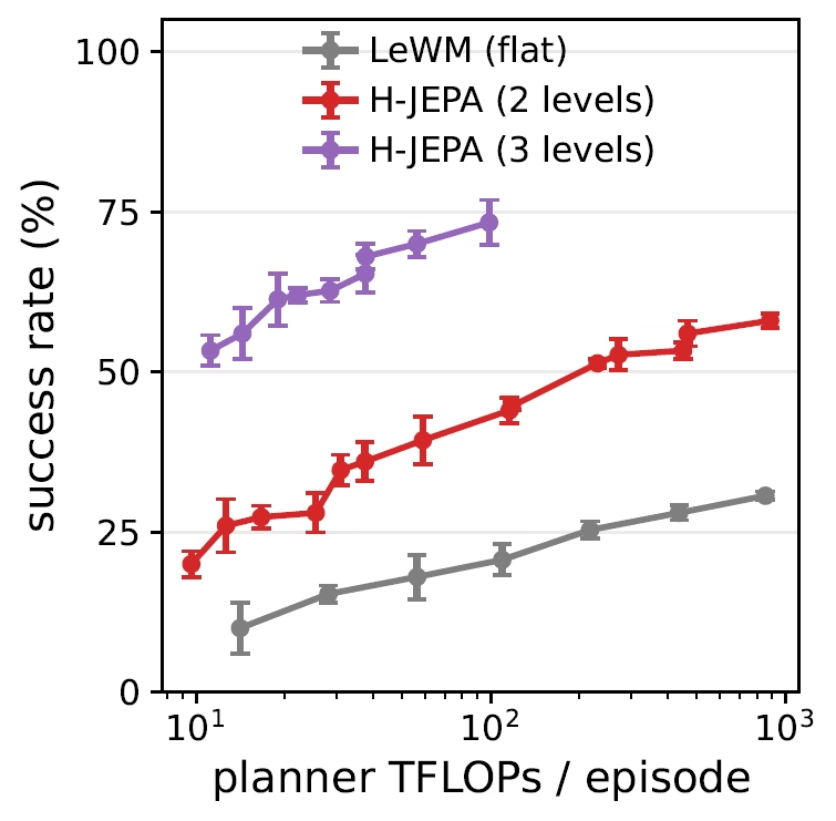
On the Visual AntMaze benchmark, the three-level H-JEPA reaches a 73% success rate, compared to just 18% for the flat LeWorldModel baseline.
We also see that it achieves this with less planning compute. So despite adding more levels to the model, the hierarchical planner can actually find better plans with less compute.
What Do Different H-JEPA Levels Learn? Visualizing the Representations
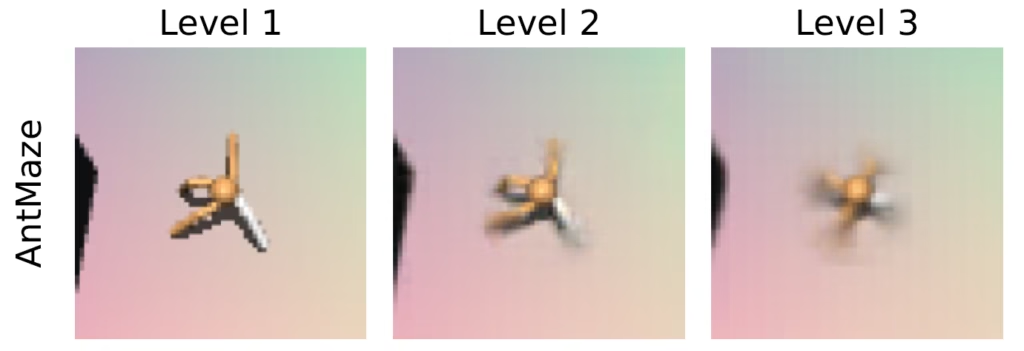
Another interesting result from the paper shows what information the different levels actually learn to retain.
To visualize this, the authors first freeze the trained world model, and then train separate decoders that turn the representations from each level back into images. These decoders are only used for visualization so they are not part of the actual H-JEPA architecture.
In AntMaze, as we move up the hierarchy, the ant’s leg pose becomes less and less distinct, but its position in the maze remains clear.
The authors hypothesize that this happens because each level is trained to predict over its own time horizon. Details that change quickly, like the ant’s leg configuration, are harder to predict far into the future. So higher levels learn to discard these details while retaining slower-changing, more predictable information, like the ant’s position.
This is useful for planning because reaching a goal usually depends much more on where the ant is than on the exact position of its legs.
References & Links
- Paper page
- GitHub page
- LeWorldModel breakdown
- Join our newsletter to receive concise 1-minute read summaries for the papers we review – Newsletter
All credit for the research goes to the researchers who wrote the paper we covered in this post.