In this post, we break down LeWorldModel (LeWM), a new stable Joint-Embedding Predictive Architecture (JEPA) world model, introduced in a paper co-authored by Yann LeCun.
Introduction
What Is LeCun’s Vision for World Models?
It’s been 4 years since Yann LeCun laid out his vision for a more human-like AI in a famous 62-page paper, A Path Towards Autonomous Machine Intelligence. At the heart of that vision sits the world model.
As humans, we carry a mental model of how the world behaves. If we push a cup, we expect it to slide. Push it too far, and we expect it to fall. LeCun says that similarly, an intelligent agent should be able to imagine the consequences of its actions before taking them.
What Is JEPA?
The architecture LeCun proposed for learning such a model is JEPA, short for Joint-Embedding Predictive Architecture.
The key idea is that JEPA doesn’t try to predict the future pixel by pixel. When we imagine pushing that cup, we don’t render a video in our heads. Instead, we reason at the level of objects and concepts. JEPA follows the same philosophy by predicting abstract representations instead of raw pixels.
The challenge is making this actually work. While the idea sounds elegant, training these kinds of models has proven unstable. We’ll see why shortly.
In this article, we cover a new paper titled “LeWorldModel: Stable End-to-End Joint-Embedding Predictive Architecture from Pixels”, with LeCun himself among the authors, that introduces a way to train a simple and stable JEPA world model, something that has been a longstanding challenge with previous JEPA models. Don’t worry if you’re not familiar with previous JEPA papers. No prior knowledge is needed to follow along.
How Does LeWorldModel Work?
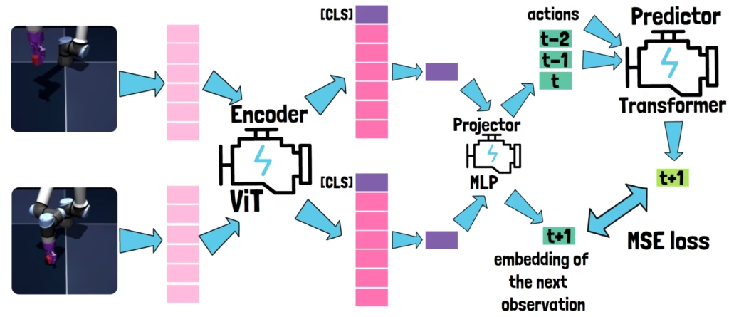
To learn how the world behaves, the model is trained on sequences of observations and the actions performed between them.
For example, on the left of the illustration above, we have two consecutive observations of a robotic arm. The action between them could be moving the arm in a certain direction or lifting an object.
The idea is using the earlier observation and the action, to predict what comes next, which is the second observation. But as we mentioned earlier, JEPA doesn’t predict future pixels. Instead, it predicts the future in a semantic representation space.
This happens in two stages:
- First, each observation is converted into a semantic representation by an encoder.
- Then, another component predicts the representation of the next observation.
The Encoder
The encoder is implemented using a Vision Transformer (ViT), a standard architecture in computer vision. Like any Vision Transformer, it first splits the image into a sequence of patches. These patches are then converted into embeddings and processed together by the Transformer.
For clarification, we note that while the encoder handles both observations, each is processed independently.
The Class Token
Each patch embedding represents a small area in the original image. However, JEPA needs a representation of the entire observation. To achieve this, the Vision Transformer adds a special token embedding called the class token.
This token is introduced at the beginning of the Transformer processing and is processed alongside all the patch embeddings. As information flows through the network, the class token gathers information from all image regions, allowing it to capture the high-level semantics of the entire observation.
Since JEPA is designed to reason at the level of concepts rather than visual details, it keeps only the class token and discards the remaining patch embeddings. The class token embedding is then passed through a projection layer to produce the final semantic representation of the observation.
Another motivation for keeping only the class token is efficiency, as it significantly reduces the input size for the next component.
The Predictor
The next component is called the predictor, modeled as a standard Transformer rather than a ViT. Its job is to predict the semantic representation of the next observation.
It can use more than just the last observation for prediction. In the illustration avove, the predictor receives the representations of the three most recent observations. Additionally, the predictor also gets the actions performed between the observations, and the current action that should lead to the next observation.
Based on this information, the predictor generates its prediction for the next observation’s representation.
How Is LeWorldModel Trained?
During training, the predicted representation is compared with the representation produced by the encoder for the actual next observation. The difference between the two is measured using an MSE loss, and both the encoder and the predictor are optimized together to minimize it.
The Model Collapse Problem
A common challenge with this kind of approach is model collapse. Instead of learning meaningful representations, the model could simply output the same embedding for every observation.
If both the encoder and the predictor always produce that constant embedding, the prediction loss becomes very small, even though the model has learned nothing about how the world behaves.
Previous approaches have relied on different techniques to prevent this collapse. For example, a DINO World Model (Dino-WM) uses a pretrained DINO encoder instead of learning the representation from scratch.
How Does LeWorldModel Prevent Model Collapse?
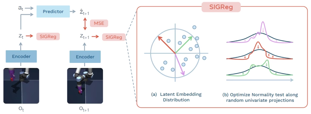
LeWorldModel takes a different approach. It introduces a simple training strategy that allows the encoder and predictor to be trained end-to-end while remaining stable. We can understand this using the above figure from the paper.
On the left, we see the architecture we just discussed, with one important addition: a second training signal on top of the prediction loss. This additional signal is a regularization term called SIGReg, short for Sketched Isotropic Gaussian Regularizer. It was also introduced by LeCun in another paper published at the end of 2025.
What Is SIGReg?
So what is this regularization term trying to do? To understand that, let’s look at the right side of the figure above.
The first plot shows a visualization of the latent embedding space. Each dot represents the embedding of one observation from a batch, with all of these embeddings plotted together as a cloud of points.
SIGReg then takes random directions through this embedding space, shown as the red, green, and purple arrows. For each direction, SIGReg projects every embedding onto that direction. This gives us a one-dimensional distribution of values. That’s what we see in the plot on the right.
For each colored direction, the colored curve shows the actual distribution we get by projecting the embeddings onto that direction. SIGReg compares this distribution with a standard normal, or Gaussian, distribution shown alongside it.
The goal is to make these two distributions as similar as possible. In other words, SIGReg encourages the embeddings to follow a Gaussian distribution along each of these random directions.
In practice, this process is repeated over many directions. Specifically, 1024 random directions are used in this paper. By doing this across many directions, SIGReg encourages the overall embedding space to become approximately Gaussian, rather than collapsing into a small region.
And this helps prevent model collapse, because the encoder is encouraged to produce a diverse, well-distributed representation of the observations instead of mapping everything to the same embedding.
So, the prediction loss teaches the model to predict what comes next, while SIGReg encourages the representation space itself to remain well-behaved.
How Does LeWorldModel Use Latent Planning?
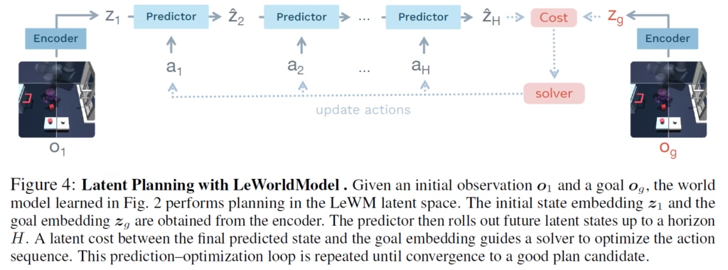
Now that we understand how LeWorldModel learns a representation of the world, the next question is how can we actually use that model to make decisions? The answer is latent planning, and we can understand how it works using the above figure from the paper.
On the left, we see an initial observation, which represents the current state of the environment. On the right, we see a goal observation, an image representing the state we want to reach.
The goal of planning is to find an action sequence that takes the environment from the initial state to as close as possible to the goal.
How Does Latent Planning Work?
We begin by randomly sampling many different possible action sequences. For each sequence, the predictor uses the learned world model to imagine where those actions would take us, by predicting the future observation representations step by step.
We then compare the final imagined representation with the representation of the goal observation. The difference between them gives us a cost. The lower the cost, the closer our imagined outcome is to the goal.
This cost is then used to update the action sequence distribution, making action sequences that lead to better outcomes more likely to be selected in the next iteration.
This process is then repeated until a satisfied cost is obtained when we reach a good plan.
Importantly, the model doesn’t have to commit to the entire plan. Instead, it can execute only the first few actions, observe the new state of the environment, and then plan again from that new state.
How Does LeWorldModel Perform?
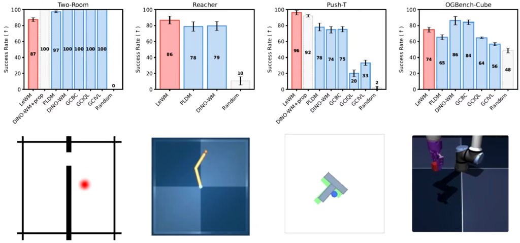
The above figure shows the planning performance across four environments:
- Two-Room: The simplest of the four, where an agent has to navigate from one room to another to reach a target location.
- Reacher: A two-jointed robotic arm that has to align itself with a target position.
- Push-T: The agent has to push a T-shaped block into a target configuration.
- OGBench-Cube: A 3D robotic arm task where the arm has to pick up a cube and place it at a target position. It’s also the most visually complex environment of the four.
LeWorldModel vs. the Baselines
The results are quite interesting.
On Push-T and Reacher, LeWorldModel outperforms the baselines. LeWorldModel even outperforms a version of DINO-WM that has access to additional information the others don’t use, which is the arm’s position rather than just pixels.
On OGBench-Cube, DINO-WM performs better than LeWorldModel. The authors suggest that the higher visual complexity in this environment make learning the visual representation more challenging. DINO-WM may have an advantage here because it relies on a large-scale pretrained visual encoder, which provides richer visual embeddings.
And on Two-Room, the simplest environment, LeWorldModel falls behind the baselines. The authors hypothesize that this may be because the environment has very low dimensionality. In such a simple setting, forcing the latent space toward a high-dimensional Gaussian distribution with SIGReg may actually make the learned representation less well structured.
LeWorldModel’s Planning Efficiency
So LeWorldModel doesn’t outperform every baseline on every task. But it is worth mentioning that LeWorldModel is much smaller than the baselines. Additionally, using just the class token embedding for prediction makes its planning significantly faster. The authors report a roughly 48-times speedup.
References & Links
- Paper Page
- Code
- Project Page
- Join our newsletter to receive concise 1-minute read summaries for the papers we review – Newsletter
All credit for the research goes to the researchers who wrote the paper we covered in this post.