
In this post we dive into a new research paper from Apple titled: “LLM in a flash: Efficient Large Language Model Inference with Limited Memory”.
Before divining in, if you prefer a video format then check out our video review for this paper:
Motivation
In recent years, we’ve seen a tremendous success of large language models with models such as GPT, LLaMA and more. As we move forward, we see that the model’s size is getting larger and larger, and in order to efficiently run large language models we need a substantial amount of compute and memory resources, which are not accessible for most people. And so, an important research domain is to democratize large language models.

LLM in a flash & LLMs Democratization
The common approach to make LLMs more accessible is by reducing the model size, but in this paper the researchers from Apple present a method to run large language models using less resources, specifically on a device that does not have enough memory to load the entire model. They do so by using a novel method to load the model from flash memory in parts. This is a big deal as it is a step towards being able to run high-end large language models efficiently on devices with less resources such as our phones.
Latency Improvement Results

In the above chart from the paper, we can see the inference time of a model when using the paper method comparing to naively loading the model from flash, when half the memory of the model size is available in DRAM. And we can see that on a GPU it takes less than 100 milliseconds, comparing to more than 2 seconds with the naive method, which is more than 20 times faster! In the rest of this post we explain how this method works.
High-Level Memory Architecture
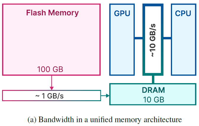
The above diagram from the paper helps to understand the relation between flash memory, DRAM and internal GPU and CPU memory. The flash memory is larger than the DRAM, in this example the flash memory has 100 GB size while the DRAM is of 10 GB size. The DRAM is usually larger than the internal memory in the GPU and CPU. However, the flash memory is slower than the DRAM. In this example, the bandwidth of the flash memory is 1 GB per second while in the DRAM we have a bandwidth of 10 GB per second.
Loading LLM Weights For LLM Inference

Say we have a LLM weights in flash memory (the purple hexagon in the above image), then for LLM inference, the standard approach is to load all of the weights into the DRAM, this can be a bit slow but it happens once, and then we pass the weights to the GPU, possibly on demand when they are needed and not all at once.
This is nice, but what happens when the available DRAM size is not large enough to store all of the model weights? Loading the model in chunks on demand from the flash memory in a naive method is very slow and can take seconds for a single inference. We saw this in results chart earlier. Ok, so what can we do to improve the inference latency in case we do not have enough DRAM size?
Improving Inference Time When Memory Is Limited
The paper suggests three areas for improvement. First let’s review the three areas and then we’ll dive into the first two.
- Reducing Data Transfer – the idea here is that we do not read the entire model from flash memory but rather load only weights that are really needed. The researchers also introduce a new method they call windowing that helps with that which we will cover soon.
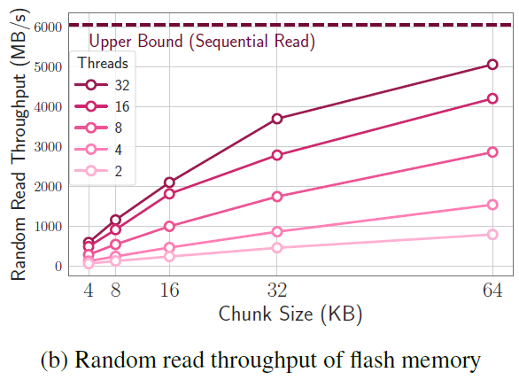
- Optimization of Chunk Size – When reading from flash memory there is an importance for the size of the chunk that we read. In the below chart from the paper, we have the chunk size on the x axis, and the read throughput on the y axis, and we can see that larger chunk size reads have higher throughput. The multiple lines are for using different number of threads.
- Smart memory management that helps to reduce overhead of copying data in the DRAM, which supports the windowing method which will cover soon.
Reduce Data Transfer
Leveraging Sparsity in FFNs
We now expand more about how we can reduce the amount of data transfer. First, in each of the transformer layers we have the attention layer and a feed forward network (FFN), and we note that the attention layer weights are kept in memory constantly. This constitutes about one third of the model weights. So, the dynamic loading is related only to the FFN weights, and FFNs tend to be extremely sparse. So, we want to dynamically load the non-sparse segments to DRAM, when they are needed.
Windowing

The dynamic loading is done using windowing, which we can learn about from the above figure from the paper. Instead of feeding all of the input sequence to the FFN, we only feed it with a window from the sequence, in this example of size five. When feeding the network with a window, we load the weights which we expect to not be zeroed out. Now, when we move the window by one, and predict which neurons are active, most of the active neuron will be shared from the previous window, so there is only need to load small amount of weights, which are marked with blue and deleted ones are marked with red.
Window Size Tradeoff With Loaded Memory
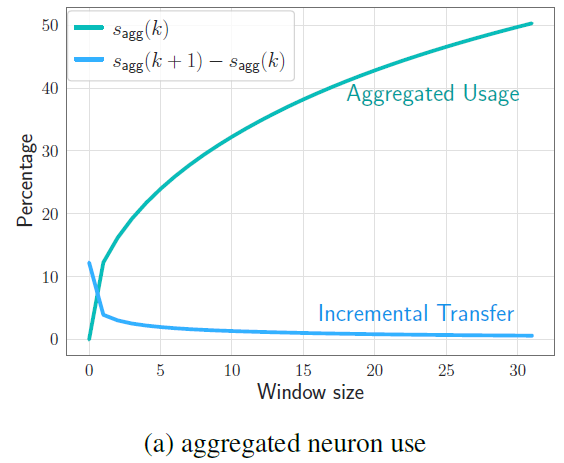
An interesting observation here can be seen in the above chart from the paper, where on the x axis we have the window size, and on the y axis we have the percentage of the model’s weights that are loaded to the DRAM. In the upper line we see that for larger window sizes, we have larger portion of the model loaded into the memory, and on the bottom line we see that as the window size grows, we have less weights needed to be loaded in each step when the window moves to the next token in the input sequence.
Optimizing Chunk Size
Earlier we saw the increasing the chunk size can help to improve the flash memory read throughput. The researchers were able to increase the chunk size using a method they call bundling columns and rows.
Bundling Columns And Rows

When using a neuron, it means that we need its respective column from the previous layer and its respective row from the next layer, so we will have to load both the column and the row from flash to DRAM. So, storing them together in flash memory, as we can see in the above diagram from the paper, helps to increase the size of the chunk we read, instead of reading two separated chunks. So, we both reduce IO requests and increase chunk size here.
Bundling Based on Co-activation
Another method that the researchers have tried and did not work is bundling based on co-activation, where the researchers showed that neurons tend to activate together with other same neurons. The researchers have decided to create a bundle in flash memory of each neuron with the one it activates with most of the times, and load them together when any of them is used. However, the results in this case showed that neurons that are very active tend to be used in most of these bundles and thus loaded many times redundantly.
References & Links
- Paper page – https://arxiv.org/abs/2312.11514
- Video – https://youtu.be/nI3uYT3quxQ
- Join our newsletter to receive concise 1 minute summaries of the papers we review – https://aipapersacademy.com/newsletter/
All credit for the research goes to the researchers who wrote the paper we covered in this post.