In this post we dive into Consistency Large Language Models, or CLLMs in short, which were introduced in a recent research paper that goes by the same name.

Before diving in, if you prefer a video format then check out the following video:
Motivation
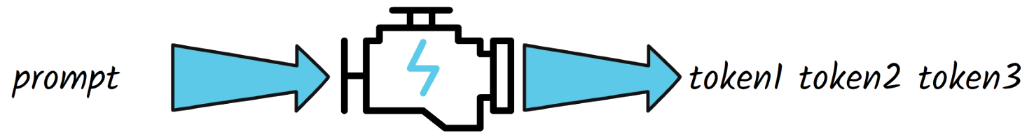
Top LLMs such as GPT-4, LLaMA3 and more, are pushing the limits of AI to remarkable advancements. When we feed a LLM with a prompt, it only generates a single token at a time. In order to generate the second token in the response, another pass of the LLM is needed, now both with the prompt and the generated token,. In order to generate another token in the response, we need to do this again, now providing the LLM both with the prompt and the two generated tokens. Obviously, this behavior is causing latency when using LLMs, and so, a common research domain is to improve LLM inference latency. The paper we explain in this post shows a method to generate multiple tokens in one LLM pass, rather than token by token, and the researchers show an improvement of 2.4 to 3.4 times in generation speed, while preserving the quality!
Jacobi Decoding
The method of CLLMs is based on an existing method which is called Jacobi decoding. With this method, instead of generating a single token at a time, we generate a sequence of tokens on one pass, which is random at first, and we iteratively fix the response sequence. The path between the random starting point and the final response is called the Jacobi trajectory. To explain it, we use the below figure from the paper.
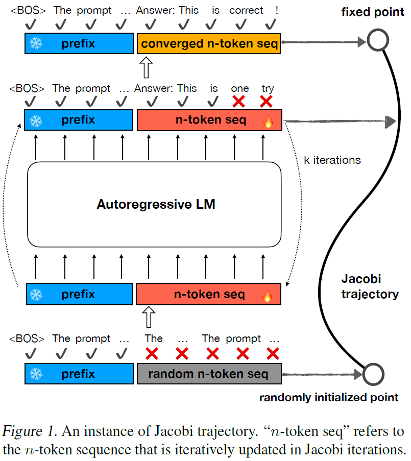
At the bottom we can see the prompt in blue, and the initial random response sequence in gray where each token is marked with a red X since it is a wrong prediction at this stage. The circle on the right represents the starting of the Jacobi trajectory. In each step, we feed the prompt and the current response sequence into the LLM, and fix every token in the response sequence if needed. It is important to mention that this is done in a single LLM pass, since we can update each token by masking out future tokens for each token that we update. After each iteration, we have more correct tokens in the response sequence than before, and another point is added to the Jacobi trajectory. After enough iterations of this, we converge into a valid response, which is the final point in the Jacobi trajectory.
Jacobi Decoding Minimal Performance Gain
In practice, vanilla Jacobi decoding not improve the latency much, and there are two reasons for that. One is that in each iteration, each LLM pass is slower, since we process also the response sequence tokens. Second is that the LLM is usually able to fix only one token from the response sequence, or a bit more on average. By the end of this post we’ll understand how this method is dramatically improved with CLLMs.
Computer Vision Analogy
The method of consistency large language models has a very strong analogy from the computer vision domain, which is improving the performance of diffusion models using consistency models.
Diffusion Models
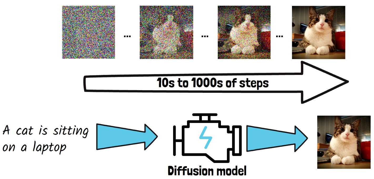
Diffusion models are the backbone architecture behind the top text-to-image generation models. Diffusion models get a prompt as input such as “A cat is sitting on a laptop”. The model learns to gradually remove noise from an image in order to generate a clear image. The model starts with a random noise image like we have above on the left, and in each step, it removes some of the noise, and the noise removal is conditioned on the input prompt, so we’ll end with an image that match the prompt. The 3 dots imply that we skip steps in this example. Finally, we get a nice clear image of a cat, which we take as the final output of the diffusion model for the provided prompt. The noise removal process usually takes between 10s to 1000s of steps, so it comes with a latency drawback.
Consistency Models
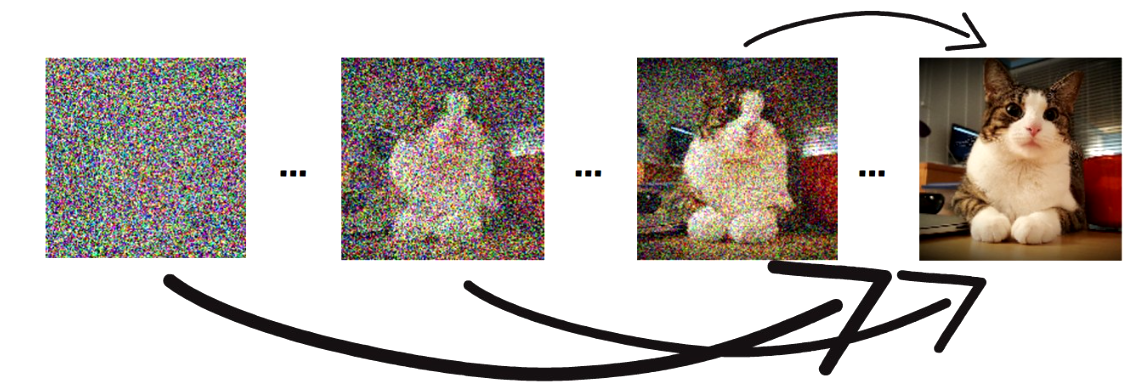
To avoid the latency drawback of diffusion models, consistency models were invented. Consistency models reduce the number of iterations required to remove the noise from an image. So, what are consistency models? Consistency models are similar to diffusion models in the sense that they also get a prompt and learn to remove noise from an image, so in the example above we have the diffusion path of a cat image, same as before. However, consistency models learn to map between any image on the same denoising path, to the clear image. So, we call them consistency models because the models learn to be consistent for producing the same clear image for any point on the same path. With this approach, a trained consistency model can jump directly to a clear image from a noisy image. In practice, few iterations of denoising are needed here as well, but just a few, much less than with diffusion models.
Consistency Large Language Models
We finally now get to understand how consistency LLMs improve the performance of LLMs.
Creating a Jacobi Trajectories Dataset
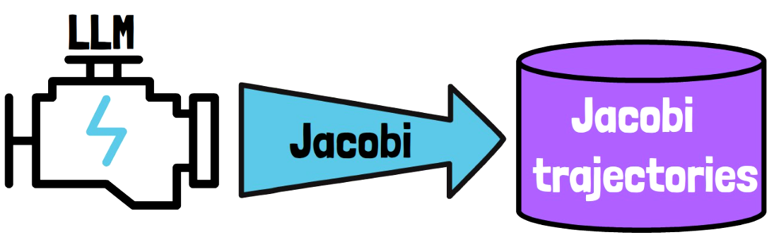
The first step is to create a dataset of Jacobi trajectories. We do that by taking a pre-trained LLM and run Jacobi decoding as we’ve seen earlier over as much prompts as we want.
Fine-tune The LLM On Jacobi Trajectories
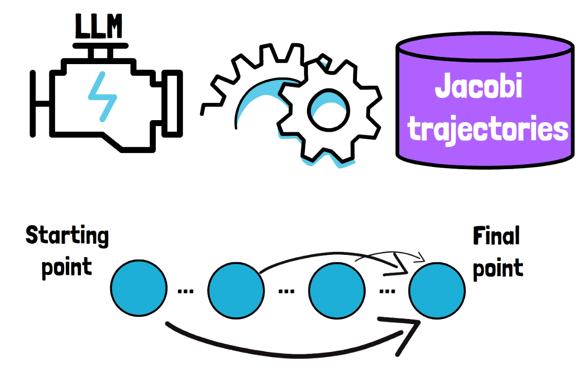
Now that we have such a dataset, we look at a Jacobi trajectory for example. And similar to consistency models for diffusion models, here as well we train the model to yield the final point in the Jacobi trajectory from each of the intermediate points. Which model do we train? The same LLM that we’ve used to create the Jacobi trajectories dataset.
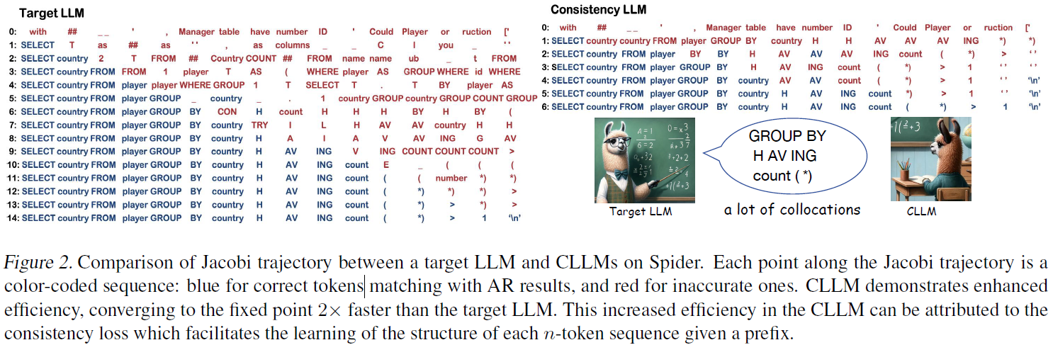
CLLMs Inference Process
To produce outputs from CLLMs, we run a Jacobi decoding, but we replace the regular LLM with a CLLM which was trained over Jacobi trajectories, and this way significantly speed up the decoding process. In the following figure from the paper, we see an example for how such a decoding may look like for a standard LLM and a consistency LLM, where blue tokens are correct and red ones are wrong. On the left we see a Jacobi trajectory for a standard LLM, showing 14 steps until all tokens are correct, and on the right, we see a Jacobi trajectory for a consistency LLM which only has 6 steps.
Results
Let’s now also take a look at a quantitative comparison for 2 of the evaluated datasets. There are more available results in the paper which we do not cover here.
GSM8K
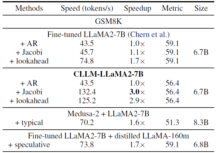
In the above table from the paper, we see a comparison over the math dataset GSM8K. In the first row we have a standard LLM we compare to. By just using Jacobi with standard LLM we see there is no significant speedup. We did not talk about lookahead in this post, but this is another improvement that is using Jacobi decoding. In this case it achieves a speedup of 1.7. When looking at the CLLM results, we see it is 3 times faster than the original LLM, and we pay a bit in performance which is 56.4 comparing to 59.1 before. Medusa is a different method to predict multiple tokens at once, which we see performs worse in this case, and also that the model size is larger. Speculative decoding achieves identical performance, with a speedup of 1.7, but here as well the model architecture is not identical to the original LLM as with CLLM.
ShareGPT (MT-Bench)
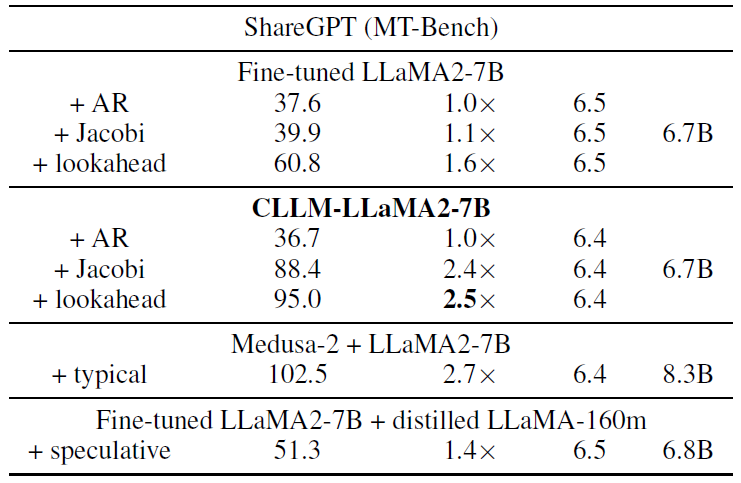
In the above table from the paper, we see a comparison on the MT-Bench dataset, where here we see that Jacobi with CLLM achieves 2.4 speedup with just a slight decrease in performance. Medusa achieves a bit better speedup in this case, but again we pay for a larger model size with Medusa. Speculative decoding again achieves an identical performance, but with a lower speedup.
References & Links
- Paper page – https://arxiv.org/abs/2403.00835
- GitHub page – https://github.com/hao-ai-lab/Consistency_LLM
- Join our newsletter to receive concise 1 minute read summaries of the papers we review – https://aipapersacademy.com/newsletter/
All credit for the research goes to the researchers who wrote the paper we covered in this post.