From Sparse to Soft Mixture of Experts

In this post we will dive into a research paper by Google DeepMind titled “From Sparse to Soft Mixtures of Experts”.
In recent years we see that transformer-based models are getting larger and larger in order to improve their performance. An undesirable consequence is that the computational cost is also getting larger.

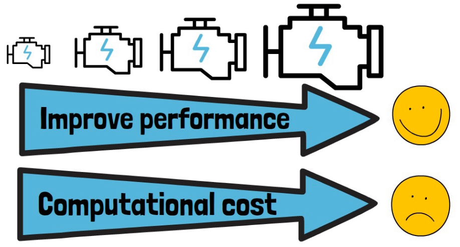
Transformer-based models are getting larger, improving their performance but also their computational cost

And here comes mixture of experts which helps to increase the model capacity without paying the full computational cost, and based on reports, it is also used by OpenAI as part of GPT-4 architecture.
However, this method also has drawbacks which the new method presented in the paper helps to resolve. In this post, we will explain the paper and understand how Soft Mixture of Experts (Soft MoE) method works and how it compares to the common Sparse Mixture of Experts.
But first, it is important to understand what is Mixture of Experts (MoE).

If you prefer a video format, then most of what we are going to cover here is also covered in the following video:

Sparse Mixture of Experts

The common methods up until now are called Sparse Mixture of Experts (Sparse MoE). The idea with mixture of experts is that instead of having one large model that handles all of the input space, we divide the problem such that different parts of the input space are handled by different experts. What does it mean?

Sparse MoE High-Level Architecutre. Passing a token via the router and chosen experts — Sparse MoE – Passing a token via the router and chosen experts

In high level, we have a router component and an experts component, where the experts component is comprised of multiple distinct experts, each with its own weights. And given input tokens such as the 8 tokens we see on the left in the picture above, each token passes via the router, and the router decides which expert should handle this token, and routes the token to be processed by that expert. More commonly, the router chooses more than one expert for each token, as in the example in the picture above where we choose 2 experts out of 4. The chosen experts then yield outputs which we combine together to reach a combined result.
These experts can be smaller than if we would use one large model to process all tokens, and they can run in parallel, so this is why the computational cost is reduced.

Sparse MoE - Passing another token via the router and chosen experts — Sparse MoE – Passing another token via the router and chosen experts

This flow is repeated for each input token. In the picture above we can see the second token also passes via the router. The router can choose different experts for the second token, for example here it chose the top expert, same as for the first token, and the third expert instead of the last. And it goes on for each input token.
Of course, the tokens are handled together so this process runs in parallel for all input tokens and not one after the other as explain here for simplicity.
The are various techniques to implement the routing logic which we won’t dive into here, but it is important to say that since we choose specific tokens to pass, it requires to solve a discrete optimization problem which is hard and this is causing issues with training and makes it hard to scale up the number of experts, and here comes Soft Mixture of Experts!

Soft Mixture of Experts in High-Level

The goal of Soft Mixture of Experts (Soft MoE) is to maintain the benefits of Sparse MoE while mitigating the challenges. How does it work?

Soft MoE Partial View - Passing Tokens into the first expert — Soft MoE Partial View – Passing Tokens into the first expert

In the picture above we can see a partial view of the high-level architecture of Soft MoE. We still have the layer of experts as with Sparse MoE, and we use the same number of experts (4) for simplicity. But now, given the input tokens, instead of passing each one of them via a router component, we have a new layer which is comprised of weights for each expert, and we pass all of the input tokens via each expert weights to yield the input for the expert. In the picture we see all input tokens are passed to the top expert weights layer which yields the input for the top expert, which is of size 4 in this example. The paper refers to the size of the expert input as slots, so here we have 4 slots.
A critical distinction from Sparse MoE is that each slot in the expert input is a linear combination of all input tokens, rather than a chosen input token as in Sparse MoE. This linear combination is the outcome of the the new weights layer, which has weights per slot per expert.

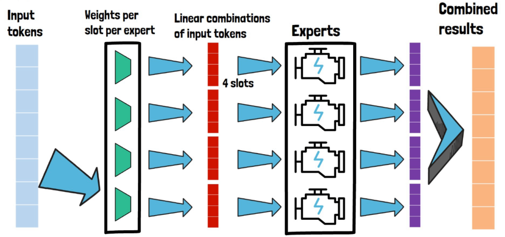
Soft MoE - High-Level Archituecture — Soft MoE – High-Level Archituecture

And this process is repeated for each expert, as we can see in the picture above that each expert has a 4 slot input to process. Each expert then yields an output for each of its slots, colored with purple in the picture. The experts results are then combined together to yield a result in the same size of the input tokens, and we know how much each expert should contribute to each slot in the final result based on the relative weight this token got from the first step. Meaning that when we created a linear combination of the input tokens in the new weights layer, then in each linear combination each token impacted the expert based on its relative weight in the linear combination comparing to other tokens, so if a certain token had high impact on a certain expert, we will want to consider the expert result for this token with higher relative weight in the combined result.
The final output can then be chained to another similar layer.

Soft Mixture of Experts Layer

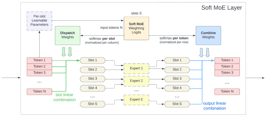
To make this new method more clear, let’s also review a diagram from the paper. In this diagram we see what happens inside a Soft Mixture of Experts layer. On the left we see we have N input tokens. They are first passed via the per-slot weights to create a N X S matrix of logits where N is the number of input tokens and S is the number of slots across all experts.
Then, we softmax per slot, meaning that for each slot here we have the weight of how much is this slot going to be impacted by any token. We then create the linear combinations for each slot. In the example here each expert has two slots.
Next, the experts yield the results for each slot as we saw before. And then we combine the experts results using another softmax over the original logits, this time by token, so for each token we know how important it was for each slot and so we consider the expert slot result for each token appropriately.

Sparse MoE vs Soft MoE

Now that we have a better understanding about each of the methods, to re-emphasize the difference between Sparse MoE and Soft MoE, consider the left side of this picture from the paper for Spare MoE, where we see that each expert has few possible slots, and we assign tokens from the input to the slots, so each expert is looking at different parts of the image here.
While with Soft MoE (on the right side of the picture), we see that similarly, the experts have slots to fill, but each one is filled with a weighted average of the input tokens. Looking at the example of a patch being assigned to a slot, for the Sparse MoE on the pink arrow we see the image patch as is, while for the soft MoE with the red arrow we see that it is a mix of the different image patches.
Unlike Sparse MoE which requires assignment between tokens to experts, all of the operations in soft MoE are continuous and fully differentiable which helps to solve some of the training issues. This is possibly also what helps this method to scale up the number of experts. If this method will be applied successfully to large language models it can be a driver to improvement over GPT-4 which is using mixture of experts according to reports. Additionally, while in sparse MoE, a token can not be assigned to any expert, or one expert could be assigned with much more tokens than other experts, here all tokens are taken into account in each expert so there is no token dropping or expert unbalance.

Results

To show the great potential of this method let’s see some of the results from the paper.

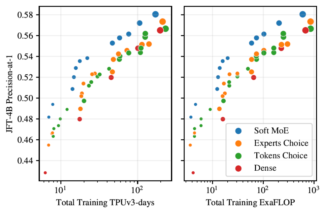
They run extensive experiments in visual recognition and starting with JFT-4B, which is an internal google images dataset, they show in the chart the performance of Soft MoE in blue, and other MoE methods in orange and green, and dense visual transformer (ViT) in red. The x axis on the left chart is TPU days and on the right chart is ExaFLOPs and it is clear that given same allocation of resources, Soft MoE outperforms visual transformer and other MoE methods.

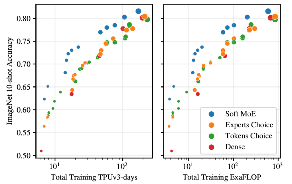
Results comparison on ImageNet of Soft MoE comparing to Sparse MoE and dense ViT

A similar trend is observed when they measure the results on ImageNet as we can see on these two charts on the right.
In order to dive deeper into the comparison of soft MoE vs dense ViT, the paper include the following table.

Looking at the largest model of both methods, a noticeable achievement here is that the inference time is much faster with Soft MoE, while results are slightly better. However, the memory footprint of running Soft MoE seems significantly larger.

References

Paper page – https://arxiv.org/abs/2308.00951
Code – https://github.com/google-research/vmoe
Video explanation – https://youtu.be/rae0Eal8ZHA