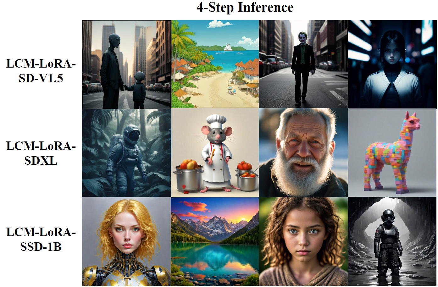
Recently, a new research paper was released, titled: “LCM-LoRA: A Universal Stable-Diffusion Acceleration Module”, which presents a method to generate high quality images with large text-to-image generation models, specifically SDXL, but doing so dramatically faster. And not only it can run SDXL much faster, it can also do so for a fine-tuned SDXL, say for a specific style, without going through another training process. In this post we’ll review the diffusion models architecture development journey from diffusion models up until now to understand how did we get here, and then explain what’s new with LCM-LoRA that made this acceleration possible.
If you’d like to receive concise one minute read summaries of the papers we review, consider to join our newsletter.

If you prefer a video format, then check out our video:
Diffusion Models
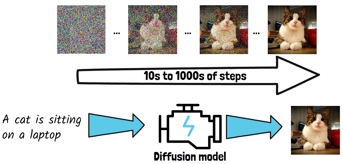
Let’s start with diffusion models. Diffusion models are the backbone architecture behind the top text-to-image generation models. Diffusion models get a prompt as input such as “A cat is sitting on a laptop”. The model learns to gradually remove noise from an image in order to generate a clear image. The model starts with a random noise image like we have above on the left, and in each step, it removes some of the noise. The noise removal is conditioned on the input prompt, so we’ll end with an image that match the prompt. The 3 dots imply that we skip steps in this example. Finally, we get a nice clear image of a cat, which we take as the final output of the diffusion model for the provided prompt. The noise removal process usually takes between 10s to 1000s of steps, so it comes with a latency drawback. In training, in order to learn how to remove noise, we gradually add noise to a clear image, which is the diffusion process.
Consistency Models

To avoid the latency drawback, consistency models were invented. Consistency models reduce the number of iterations required to remove the noise from an image. Consistency models are similar to diffusion models in the sense that they also get a prompt and learn to remove noise from an image, so above for example we have the diffusion path of a cat image, same as before. However, consistency models learn to map between any image on the same denoising path, to the clear image. So, we call them consistency models because the models learn to be consistent for producing the same clear image for any point on the same path. With this approach, a trained consistency model can jump directly to a clear image from a noisy image. In practice, few iterations of denoising are needed here as well, but just a few, much less than with diffusion models. Consistency models as originally invented, were trained by distilling information from a large pre-trained diffusion model that serves as a teacher, into the consistency model, which has its own weights.
Latent Diffusion Models (LDMs)
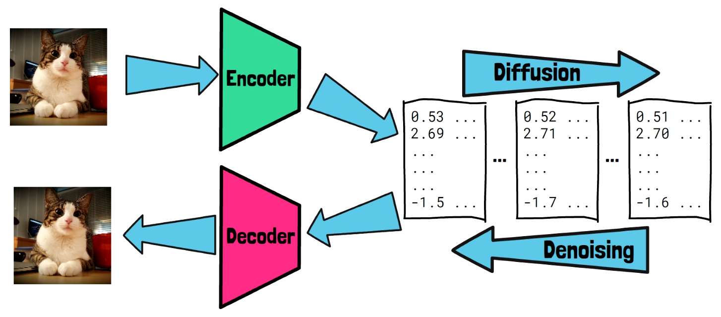
Ok, so consistency models can help to reduce the image generation latency. However, another challenge when working in the pixel space, is to generate high quality images. So here comes latent diffusion models (LDMs) which operate in a latent space, which is smaller than the pixel space. To train a latent diffusion model, we take a clear image and first pass it via an encoder. The encoder yields a representation for the image in the latent space, that preserves the image semantics. Then, the diffusion process happens in the latent space, where a noise is gradually added to the image representation. The model learns to remove the noise in the latent space, going in the backward direction. The final representation in the latent space after denoising is passed via a decoder, that yields the result in the pixel space. Doing most of the work in the latent space makes the process more efficient and allows generation of high-quality images.
Latent Consistency Models
In LDMs, similar to diffusion models, we have a generation process with many iterations. In order to optimize the generation process, latent consistency models or LCMs were introduced. Latent consistency models, similarly to consistency models, learn to directly remove all of the noise in order to skip steps in the denoising process. Unlike consistency models which were newly trained models with different weights from the diffusion models, latent consistency models are created by converting a pre-trained latent diffusion model weights into a latent consistency model. Latent consistency models we can generate high quality images in few iterations. However, training a latent consistency model requires tuning of the latent diffusion model weights. This makes it hard to convert large latent diffusion models such as SDXL to latent consistency models since they have a large amount of weights, which makes this a costly process. Additionally, we need to re-run this costly process for each style tuned version that we need.
LCM-LoRA
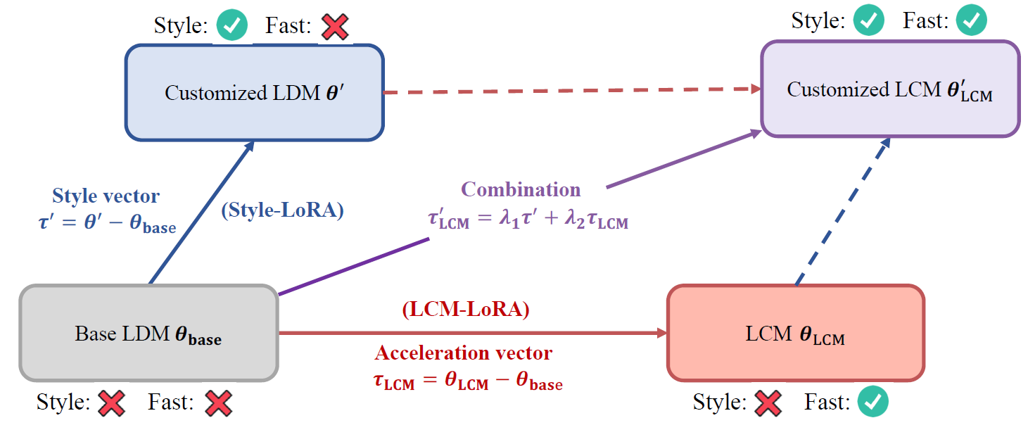
Following the challenges with creating latent consistency models without enough resources, LCM-LoRA helps to democratize this process. Instead of converting the entire stable diffusion weights, we use LoRA, meaning that small number of weights are added to the model layers, and only the added adapter weights are changing while all the pre-trained weights are kept frozen. With this method the researchers were able to convert SDXL and get high quality output in just few iterations such as the examples we saw in the beginning. Another cool attribute of LCM-LoRA is that it is possible to plug the LoRA weights to other style tuned versions of the model, so it acts as an acceleration module for Stable Diffusion models. We can see a description for that in the above figure from the paper, where on the bottom left, we have pre-trained latent diffusion model, and on the upper left we have a customized version of that model to a specific style, fine-tuned using LoRA. On the bottom right we have the LCM-LoRA version of that model. We can combine the LoRA weight from the style LoRA and the LoRA weight from LCM-LoRA and get a customized LCM version of the model without additional training.
References & Links
- LCM-LoRA paper page – https://arxiv.org/abs/2311.05556
- Video – https://youtu.be/VjmMwu1HPfw
- Join our newsletter to receive concise 1 minute summaries of the papers we review – https://aipapersacademy.com/newsletter/
- We use ChatPDF to analyze research papers – https://www.chatpdf.com/?via=ai-papers (affiliate)
All credit for the research goes to the researchers who wrote the paper we covered in this post.