Motivation
In recent years, we use AI for more and more use cases, interacting with models that provide us with remarkable outputs. As we move forward, the models we use are getting larger and larger, and so, an important research domain is to improve the efficiency of using and training AI models.
Standard MoE Is Enough?
A method which we already touched in a previous post, that became popular for large language models (LLMs), but later on also for computer vision, is Mixture-of-Experts (MoE), which helps to increase models size, without a proportional increase in computational cost. However, it comes with a large memory footprint since we need to load all of the experts. And it also does not help with the following observation.
Information Redundancy In Computer Vision
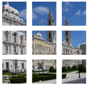
The input images in vision, which are processed as patches in vision transformers (ViTs), contain a large amount of information redundancy. For example, some of the patches, such as the one in the upper right in the image above, mostly contain background pixels. However, in vision transformers, we allocate the same compute power to all tokens, and MoE does not help with that as well.
Introducing MoNA – Mixture of Nested Experts
Both the large memory footprint, and the information redundancy, are tackled in a new method called Mixture of Nested Experts (MoNE), which is introduced in a recent research paper by Google, titled: “Mixture of Nested Experts: Adaptive Processing of Visual Token”, which we explain in this post.
Mixture of Nested Experts Layer Components
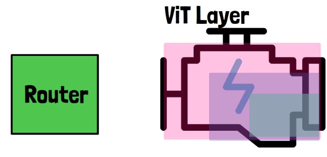
Let’s start with a high-level illustration of a mixture of nested experts layer. Later on, we will add more details. In each layer we consider two components. One is a router network, and the second is encapsulated as a regular vision transformer (ViT) layer. For this example, we define that there are 3 nested experts, marked in the imaged above with 3 different colors. One is the full vision transformer layer, another one represents a half of that layer weights, and third one represents a quarter of the weights. This is just an example and can be controlled.
The Router Assigns Probabilities To The Input Tokens
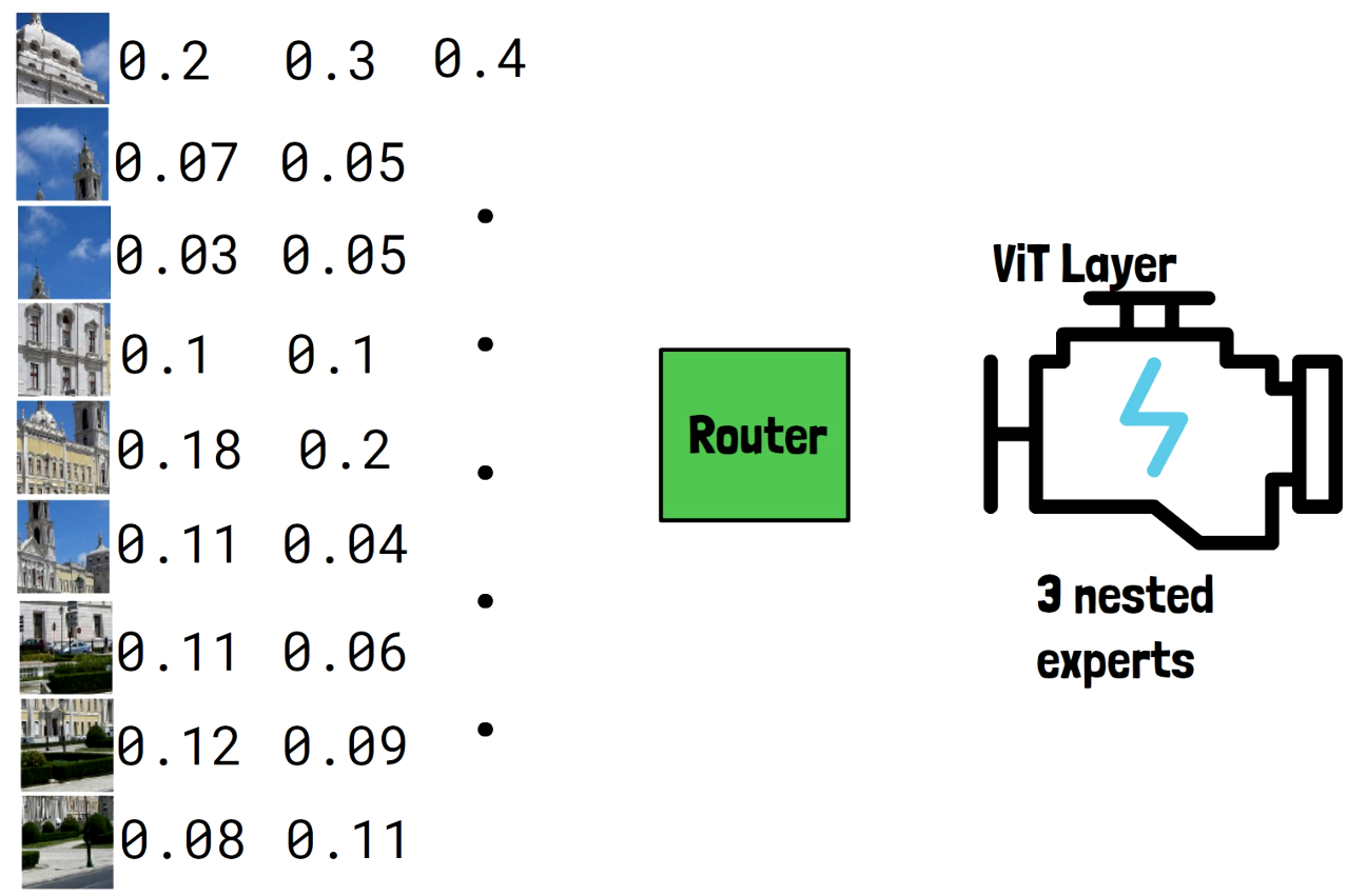
As input, we have an image divided to patches, since we use a vision transformer. The input of course is embedded to tokens before this phase. The input tokens are passed into the router, which assigns to each token, a probability to be processed by each of the experts, so, the first column of values are the probabilities to be processed by the first expert, which is the full layer. We see larger values are assigned to tokens with important information, and smaller values are assigned to tokens with less valuable information. The second column represent the probabilities of tokens to be processed by the second expert, and the third column is for the third expert.
Assigning Tokens To Experts Using Expert Preferred Routing
Once we have the probabilities, the router is using a mechanism called Expert Preferred Routing (EPR), which is presented in the paper.
Experts Tokens Capacity
Each expert has a capacity of tokens which it should process. In our example let’s assume the capacity for the first expert is 4 tokens, the second expert can process 3 tokens, and the third expert can process 2 tokens, but note that this distribution is configurable.
Assigning Tokens To The First Expert
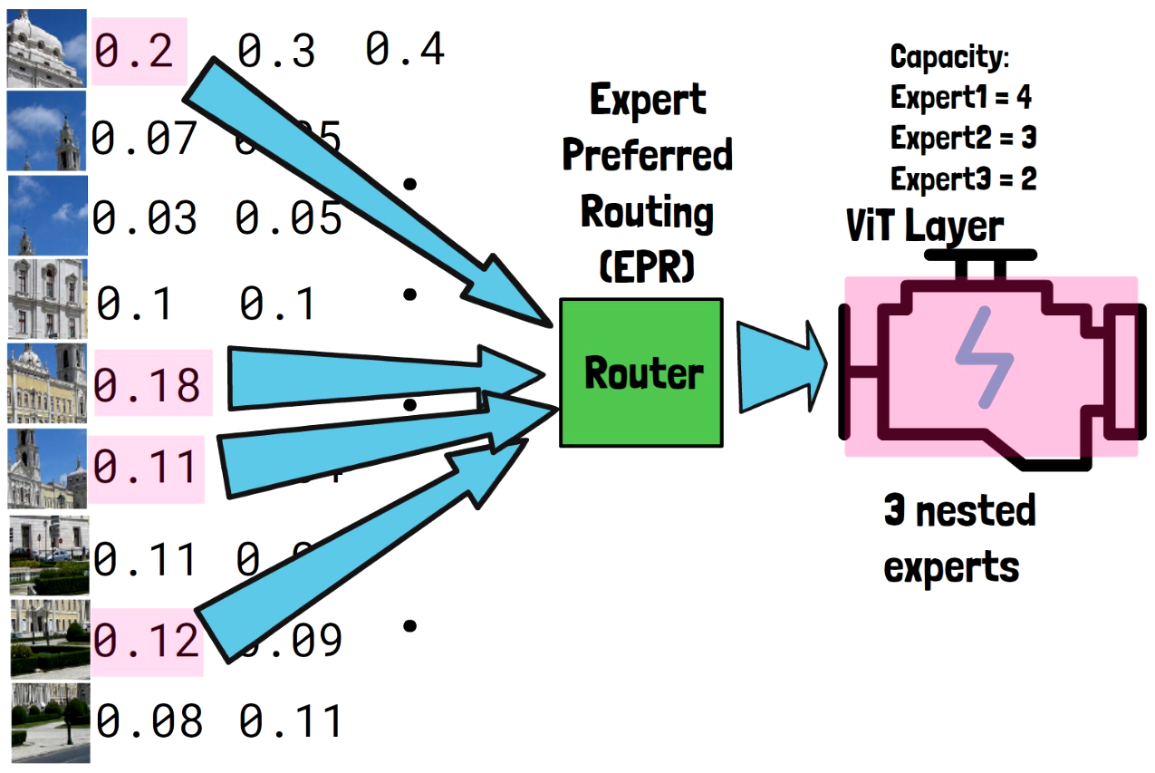
The first expert we allocate tokens to is the full layer, and the reason for that is that we want that the most important input tokens will be handled by the most capable expert, which is the first expert since it contains the full layer weights. The router takes the 4 tokens with the highest probability for the first expert, which we mark with the expert color, and routes the tokens to the first expert.
Assigning Tokens To The Second Expert
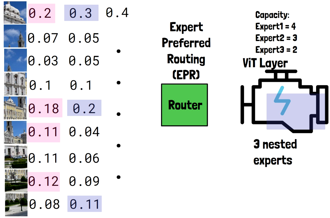
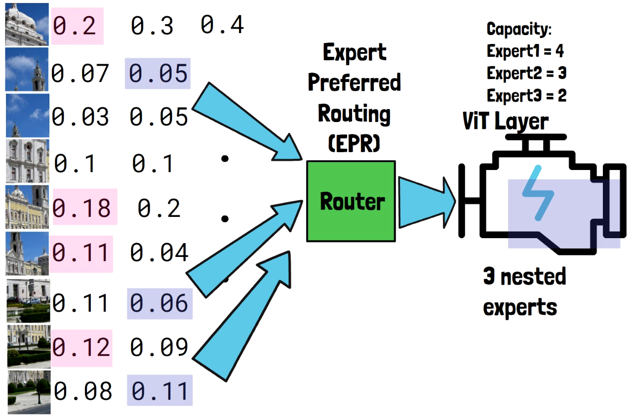
The second expert has a capacity of 3 tokens, and we mark the three tokens with highest probabilities for the second expert in the image above. We see that two out of three were already handled by the previous expert. To avoid a case where certain very important tokens are propagated to all experts, and other tokens are skipped, we limit to only select the top tokens out of the ones that were not selected yet, so instead we choose the next top two tokens, which were not yet chosen, as we can see in the image below. These three tokens are passed to the second expert via the router.
Assigning Tokens To The Third Expert
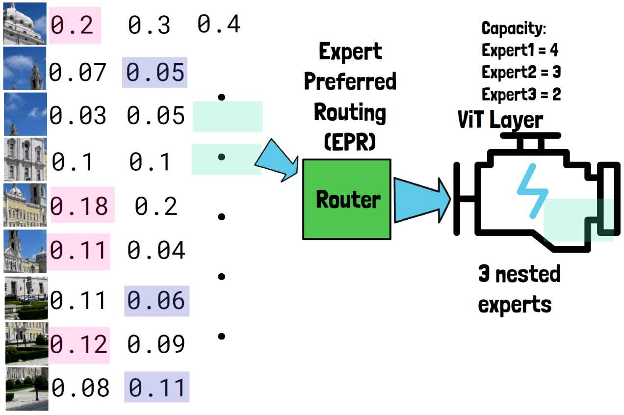
For the third expert, which has a capacity of 2 tokens, we choose the two only tokens which were not yet chosen. We do not write their probability here but it doesn’t matter because they are the only ones left. The router then routes the two tokens to the third and smallest expert, so the smallest expert handles the least important tokens.
Mixture of Nested Experts Layer Output
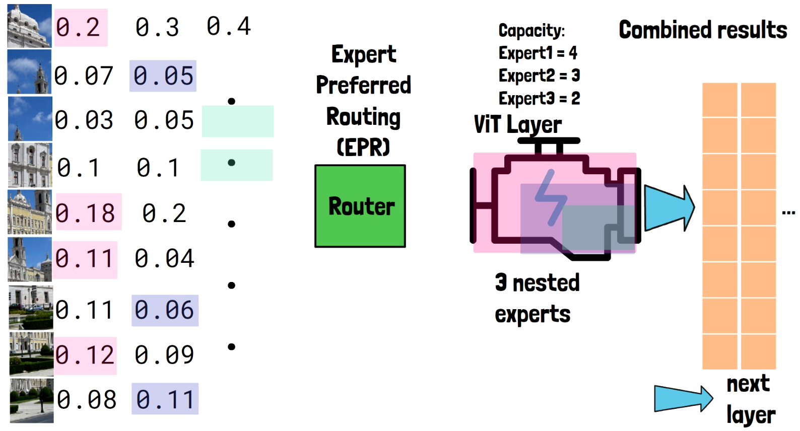
The three nested experts process the tokens that were assigned to them and the output from all nested experts is combined together. Note this is just a single layer so the output is propagated to the next layer. Another note is that tokens that are routed to nested experts which are smaller than the full layer, are downsized to the dimension of the nested expert.
Mixture of Nested Experts – A More Detailed View
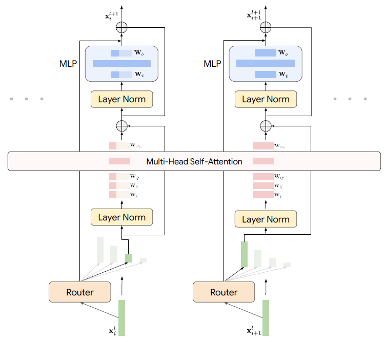
Let’s add more details by reviewing the abovefigure from the paper. We can see at the bottom two tokens that we want to process. The left one gets assigned by the router to the third expert out of 4, which we see its dimension is smaller than the full model. The token on the right gets assigned to the first expert which represents the full model layer.
Self-Attention In A Mixture of Nested Experts Layer
Both tokens, after moving via a normalization layer, reach the self-attention component. On the left, for the smaller nested expert, we see that only subset of the weights of the attention module are used to extract the query, key and value, while on the right, for the full model layer, the whole matrices are used.
However, the tokens still interact with each other in the self-attention module. This is achieved when we reach the operation that multiplies the Q, K, and V matrices together. To be able to do that, we pad the values received from smaller nested models, to the full model dimension.
MLP In A Mixture of Nested Experts Layer
After the self-attention, and another normalization step, the tokens reach the MLP module, where again on the left we see only a subset of the weights being used. So, for tokens that are routed to smaller nested models, we use less compute than for tokens that are used by larger nested models.
Results
Let’s now move on to review some of the results presented in the paper.
Mixture of Nested Experts Tokens Important Understanding
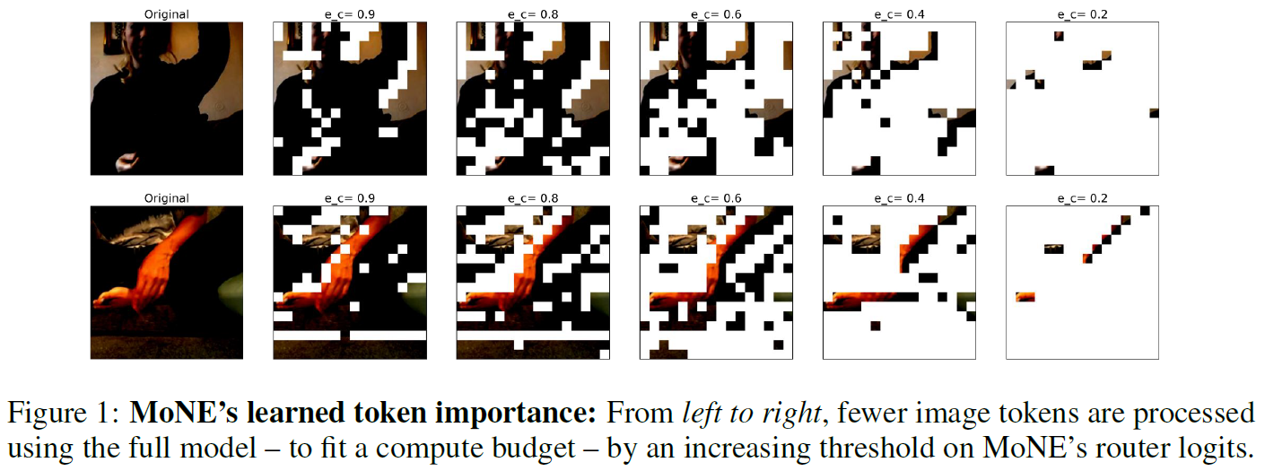
The above figure from the paper shows an example of the model ability to learn which tokens are important. On the left we have two original input images. One image to the right, we allow the full-size expert to process 0.9 of the tokens, and we see it mostly excluded less important tokens. And as we move more to the right, the full-size expert is allowed to process less and less tokens, where we more vividly see that it gets the important tokens to process. Although to be honest in the bottom image I would expect it to process more from the human hand pixels.
Image Classification Performance
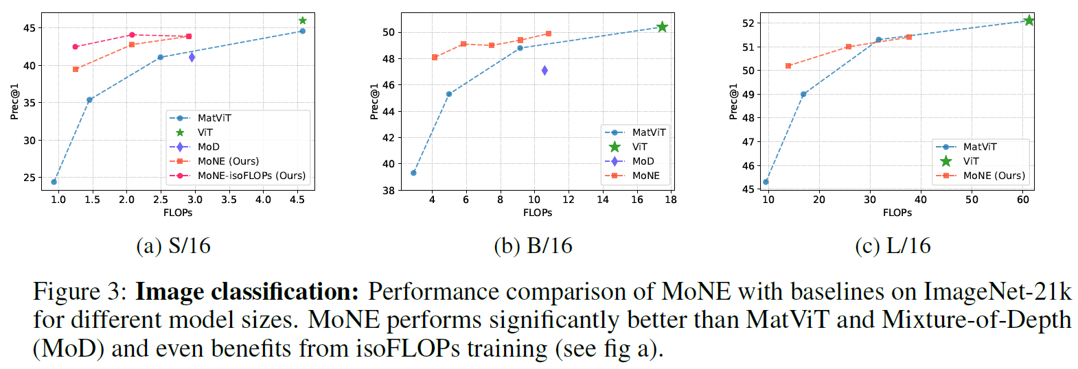
In the above figure, we can see how mixture of nested experts performs for image classification, based on the ImageNet-21k dataset. The x axis in all charts represents the compute power, and the y axis is the precision. The mixture of nested experts models are based on a vision transformer (ViT) model. The three charts are for different vision transformer sizes, small, big, and large. The vision transformer results are shown with green star. In all charts, the vision transformer is on the top right, meaning it has the best precession, but is also the most expensive to run. Then, the other models on the charts are the mixture of nested experts, in red and orange, and other related models as baselines. We see multiple dots for the mixture of nested experts models on a single chart because they are evaluated given different compute restrictions. So, in most cases when we allocate more compute power, the model is performing better. To summarize the charts, we see that mixture of nested experts can be comparable to baselines in precision, using significantly less compute.
References & Links
- Mixture of Nested Experts paper page – https://arxiv.org/abs/2407.19985
- Video – https://youtu.be/rJAndyAbErc
- Join our newsletter to receive concise 1 minute summaries of the papers we review – https://aipapersacademy.com/newsletter/
All credit for the research goes to the researchers who wrote the paper we covered in this post.