In this post, we break down Google’s Nested Learning paper and the Hope architecture, a new approach to continual learning in LLMs that aims to overcome catastrophic forgetting.
Introduction
The Memory Limitation of Modern AI
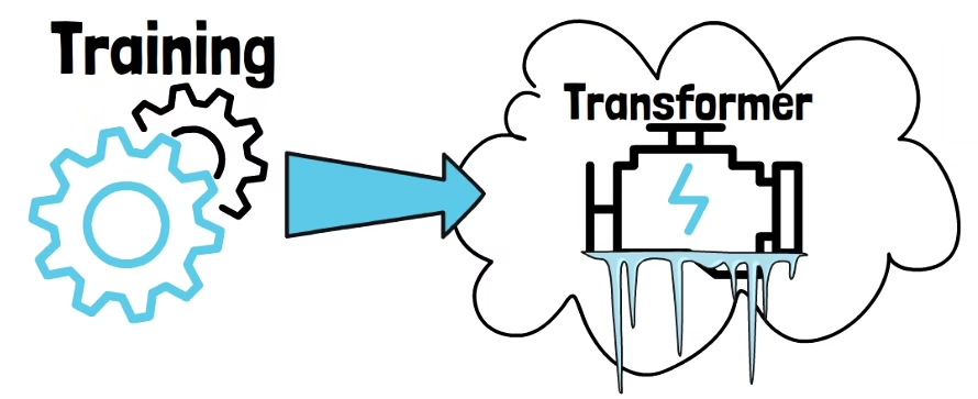
What if the biggest limitation of today’s AI isn’t intelligence, but memory? Today’s models are trained once on massive datasets, and then deployed as fixed systems.
Once training ends, these models essentially stop learning. They are frozen in time. Even though they can adapt within a conversation, that learning doesn’t last.
Transformers and the “Frozen Model” Problem
Over the last few years, progress has been driven by large language models (LLMs) powered by the Transformer architecture, which was introduced by Google in 2017 with the famous Attention Is All You Need paper.
Since then, improvements in architecture, optimization, and massive scaling have made these models far more capable, but they haven’t changed a fundamental constraint: the models still don’t continue learning after training. Attempts to keep updating them often run into a phenomenon called catastrophic forgetting, where new learning overwrites what the model already knew.
In-Context Learning vs True Continual Learning
Yes, large language models are surprisingly good at in-context learning, which is their ability to adapt on the fly based on the prompt. But this learning is not persistent. Once the context is gone, the model reverts back to its original state. In other words, the models only experience the immediate present.
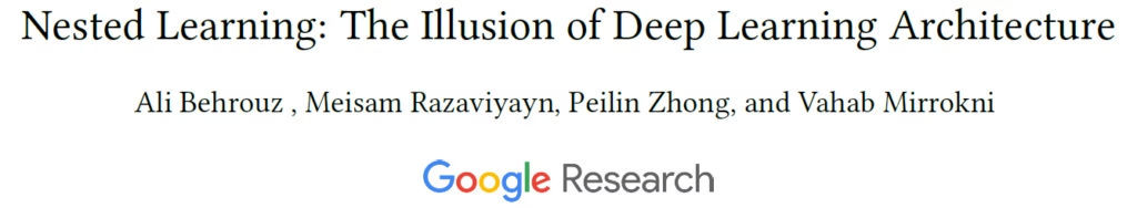
Now, Google is back with a new paper titled “Nested Learning: The Illusion of Deep Learning Architecture”, which introduces a new model architecture called Hope. And the authors’ claim is ambitious: it could rival Transformers while enabling true continual learning, without catastrophic forgetting.
Anterograde Amnesia Analogy in AI
The paper compares the issue with current large language models to a human memory disorder called anterograde amnesia. This is a neurological condition where a person can no longer form new long-term memories, while existing memories remain intact. This condition limits the person’s knowledge and experiences to a short window of present and long past, before the onset of the disorder.
To overcome this, Google proposes a new learning paradigm called Nested Learning, designed to more closely resemble how memory and learning interact in the human brain and perhaps break the “frozen in time” limitation.
Nested Learning: A Brain-Inspired Paradigm
So what aspects of human memory inspired the Nested Learning paradigm and the HOPE architecture?
The human brain is remarkably effective at continual learning. Unlike Transformers, humans continuously adapt and update their knowledge throughout life.
The paper highlights two key characteristics that enable this ability.
Neuroplasticity in Humans vs AI
The first is neuroplasticity – the brain’s capacity to change itself in response to new experiences, memories, learning, and even damage. One contributing factor to neuroplasticity is that many brain regions can be repurposed or reorganized when needed.
The paper highlights an interesting example of clinical cases where children undergo surgery removing parts of the brain to treat severe epilepsy, yet later develop largely normal cognitive abilities. These cases illustrate how neural functions can reorganize rather than remain fixed. This requires some kind of uniform structure across the brain, rather than specialized components.
Brain Oscillations and Multi-Scale Learning
The second key inspiration comes from brain oscillations, or brain waves. These are patterns of neural activity occurring at different frequencies. Different frequencies are associated with different roles. Faster oscillations, or high frequency waves, support rapid processing and short-term adaptation, while slower oscillations, or low frequency waves, are linked to long-term memory consolidation. In other words, learning in the brain happens simultaneously across multiple time scales.
Limitations of Deep Learning: Single Learning Frequency
In contrast, deep learning models typically update all parameters at the same rate during training, effectively operating at a single learning frequency. Once training ends, parameter updates stop entirely.
However, Transformers do exhibit a limited form of post-training adaptation through in-context learning. The paper interprets this as an extreme separation of time scales: The weights don’t update so they have an update frequency of 0. But the attention mechanism acts as a perfect memory for the input sequence, as it has direct access to the full sequence, without any sort of compression of data. In this sense, it can be thought of as having an infinite update frequency.
Neural Learning Modules (NLM): The Core Building Block of Hope
To understand Nested Learning, we now need to look at how the Hope model is built, and what makes it fundamentally different. But before we get there, we need to introduce an important building block called the Neural Learning Module (NLM). This is a unified building block that allows the Hope model to achieve something closer to human-like neuroplasticity and multi-scale learning.
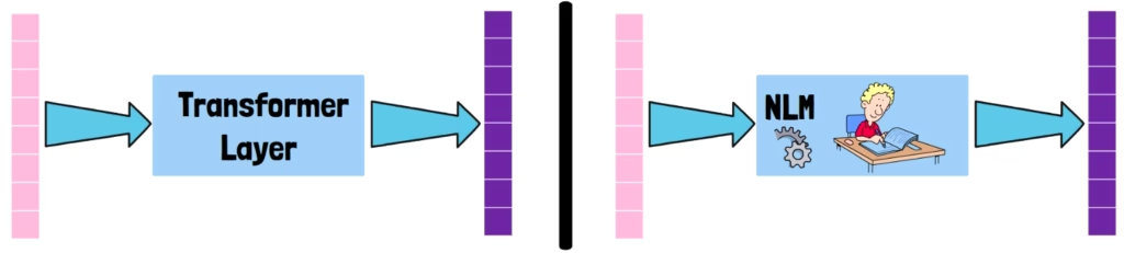
To understand the Neural Learning Module, we need to shift how we think about a layer in a neural network. In a standard Transformer, a layer is mostly static, data goes in, gets transformed, and comes out. But in the Nested Learning paradigm, a Neural Learning Module is more like a miniature student.
Instead of just passing data through, the Neural Learning Module treats the incoming information as a context flow that it must learn to compress and internalize. It does this by solving its own local optimization problem. In this sense, the Neural Learning Module behaves like an associative memory. It takes the current input and tries to memorize the relationship between that data and its local learning objective by updating its own internal weights.
As we’ll see later, a single layer in HOPE isn’t just one student, but a small classroom of them working together.
Neural Learning Module Key Properties
The Hope model is built from many Neural Learning Modules, each operating autonomously and defined by three key properties.
First, each Neural Learning Module has its own objective, a specific mathematical goal describing what it should learn from the context flow.
Second, each Neural Learning Module can have its own unique learning rate. This allows the model to decide how aggressively a specific part of its memory should change when it sees new information.
In traditional deep learning, objective and learning rate choices are global, defined once for the entire model during training. In Nested Learning, each component gets its own. For intuition, if we imagine chatting with such a model, this means that while chatting, these Neural Learning Modules are performing local mini-backpropagations in real-time, continuously refining their internal representations to compress the ongoing interaction into memory.
Third is the update frequency, inspired by brain oscillations. Frequency describes how often a Neural Learning Module updates its weights per n tokens. High-frequency modules may update their weights for every token or every few tokens to catch immediate patterns. Low-frequency modules wait until they’ve seen thousands or even millions of tokens before they consolidate that information into their weights.
The Illusion of Deep Learning Architecture
This idea of update frequencies connects to the title of the paper: The Illusion of Deep Learning Architecture. In traditional models, most parameters are updated at the same rate, effectively operating at a single time scale. The authors argue that stacking layers isn’t what truly creates depth, but rather it’s the sequence of learning updates a model goes through. In Hope, this is made explicit. Instead of stacking static layers, the model uses modules that learn at different frequencies, creating a hierarchy of learning across time.
With this building block in place, we can now look at how Google assembles these modules to create the Hope model.
Hope High-Level Architecture
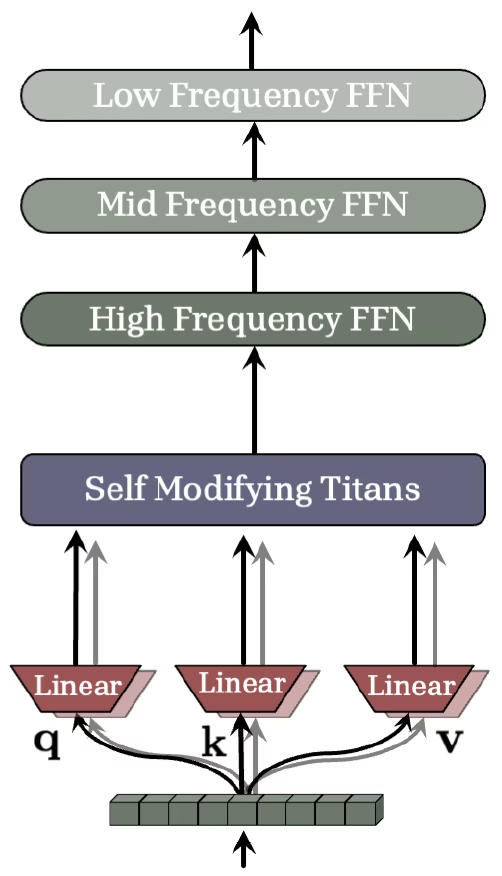
In the above figure from the paper, we can see the high-level architecture of a Hope layer. A single Hope layer is composed of two main components.
At the bottom, we start with an input sequence. Similarly to Transformers, it is projected into queries, keys and values. This is shown here in a simplified form, as we’ll see in a minute. The data then flows through two main components. The first is the Self Modifying Titans, which replace the role of attention in Transformers by handling immediate context. We’ll dive deeper into this component in a moment.
The Continuum Memory System (CMS)
The output of the Self-Modifying Titans is then processed by multiple sequential Neural Learning Modules. In practice, these are feed-forward networks operating at different update frequencies. The data is first handled by fast-updating modules and then progressively passed to slower ones.
This sequential structure is called the Continuum Memory System, or CMS. In a Transformer layer, attention is followed by a feed-forward network. In Hope, that feed-forward network is replaced by the Continuum Memory System.
How Hope Mitigates Catastrophic Forgetting
One main concern with continual learning is catastrophic forgetting, where models lose previously learned knowledge as they continue learning. The Continuum Memory System aims to mitigate that by assigning different frequencies to each module. Because each module updates at a different time, knowledge does not change everywhere at once.
This multi-frequency design creates a safety net for knowledge. If one module loses a piece of information, that knowledge isn’t gone. It still exists in other modules that haven’t updated yet. This allows important information to propagate back and be recovered.
Training The Continuum Memory System
The modules in the Continuum Memory System are trained using a global task objective, so for language modelling they are updated using a next-token prediction objective, similar to standard language models.
The Hope Architecture – A Nested Learning View
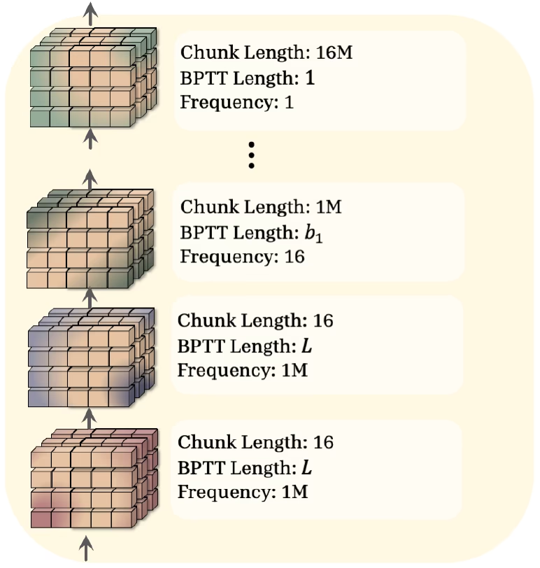
Another interesting figure from the paper shows the Nested Learning view of the Hope model as a hierarchy of Neural Learning Modules operating at different time scales.
Nested Learning View – Input Projection & Self-Modifying Titans
At the bottom are the highest frequency components: the input projection and the Self-Modifying Titans. These update very frequently. The chunk length of 16 means that these are updated after every 16 tokens. A component’s frequency describes how often it learns relative to the slowest learner in the system. The slowest learner is updated every 16 million tokens, so the 1 million frequency value means 1 million updates per 16 million tokens.
The figure also shows BPTT length. This stands for backpropagation through time. This comes from recurrent neural networks, and the Hope model is indeed a recurrent model.
In traditional recurrent networks, a hidden state, usually a vector, is updated over time. In Hope, the hidden state is the model’s own weights, which are updated using an optimizer rather than a fixed update rule.
The backpropagation through time length determines how far back gradients are propagated when learning from a sequence. For the Self-Modifying Titans, this spans the entire input sequence of length L.
Nested Learning View – The Continuum Memory System
The following Neural Learning Modules form the Continuum Memory System. These are updated much less frequently. The first is updated every 1 million tokens, while the slowest one is updated every 16 million tokens. Respectively, the frequencies are 16 and 1. Unrolling gradients across such long histories would be computationally infeasible. Therefore, the lowest frequency module has a backpropagation through time length of one, meaning it does not unroll through past tokens at all. However, its update contains information from past tokens, as it is being accumulated over time, between two updates.
For intermediate modules in the Continuum Memory System, a hyperparameter controls the tradeoff between computational efficiency and capturing longer sequential dependencies.
Self-Modifying Titans Deep Dive
Now that we have a better understanding of Hope’s high-level architecture, let’s dive deeper into what happens inside the Self-Modifying Titans.
The Titan block has two processing pathways: a retrieval pathway, which produces the current output, and a self-modification pathway, which updates the system itself. Let’s begin with the retrieval path.
Self-Modifying Titans – Retrieval Flow
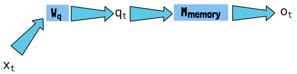
On the left, we start with our input token x_t. In practice, the sequence is processed in chunks, but here we focus on a single token for simplicity.
The input token is first projected into a query vector q_t using a projection matrix W_q. This query is then passed via a memory module denoted M_memory. The role of this module is to serve as the active memory of the input sequence. The architecture used for this memory in Hope is a 2-layer MLP.
In the retrieval pathway, nothing is updated yet. The query simply retrieves the most relevant information from the current state of the memory. This retrieved information becomes the output of the Titan at this step.
Self-Modifying Titans – Self-Update Flow
Now that we understand how the output is generated, we can expand on the self-modification pathway of the Self-Modifying Titans.
In the Nested Learning paradigm, every module is updated using its own internal objective. For the Titan’s memory, that objective is to behave as an associative memory that memorizes the input sequence.
To do this, it uses an L2-regression loss, defined by the following formula. This loss teaches the model to map between keys and target values.
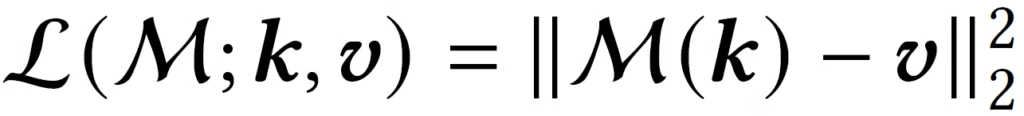
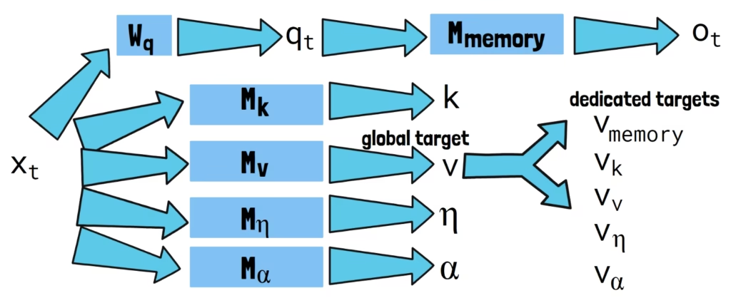
Constructing The Keys and Values
To construct these keys and values, the input is processed through a dedicated module for each. These modules are Neural Learning Modules, so unlike Transformers, where keys and values are fixed projections, here they are generated by adaptive components that evolve over time and through the processing of the input sequence.
To calculate the first part of the loss, the keys are passed via all updated modules. But for the second part of the loss, currently we only have a single global target value. The value is the target which the model tries to memorize, so to allow better adaptability, we convert this global target value into dedicated target values for each of the modules, allowing each component to learn its own representation of the input. This is done by passing the global value via the modules themselves. The loss is then calculated between the processed keys and the dedicated target values.
But the self-adaptation goes even further. The optimizer itself, the mechanism that updates the memory, is also learned.
Learning How To Learn
The model dynamically generates its own learning rate and decay factor using dedicated modules. The learning rate controls how aggressively new information is incorporated, while the decay factor determines how much past memory is retained or forgotten.
Both of these modules are also self-adaptive, so they also generate their own values for the loss calculation. This also means that the Self-Modifying Titans component learns how to update itself.
Global Task Alignment
Importantly, this entire self-modification process is self-guided. Each module decides what to store based only on the input it sees, rather than the global task objective. To ensure alignment with the global task, the initial states of these modules are trained using the global loss.
Hope Results
Needle In A Haystack
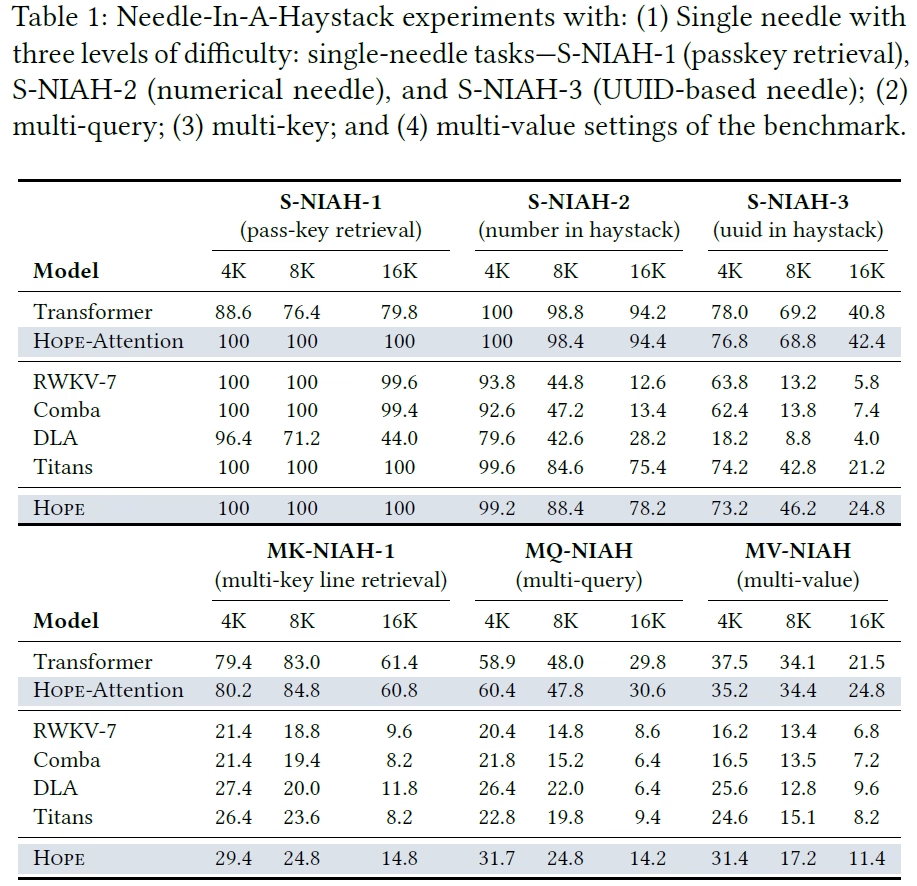
In the above table, we can see the model performance on needle in a haystack tasks. These tasks require the model to retrieve a small piece of information hidden inside a long input sequence. In the upper two rows, we can see that Hope clearly outperforms the Transformer model. The model called Hope-Attention is using an attention block instead of the Self-Modifying Titans. Therefore, the improvement can be attributed to the Continuum Memory System in this case.
Compared to recurrent baselines, Hope also shows strong gains. At the bottom row we can see the results of the Hope model with the Self-Modifying Titans, which also outperforms the Transformer model, but doesn’t outperform the Hope-Attention model.
The authors explain this result by noting that attention effectively acts as a perfect memory, since it can cache all past tokens without compressing them. Because of this, parametric models like Hope, which must compress information into their weights, are not expected to outperform attention on pure recall tasks like this.
That said, without the attention block, standard Hope avoids the quadratic cost of attention, making it much more scalable to long sequences.
Language Modeling and Reasoning
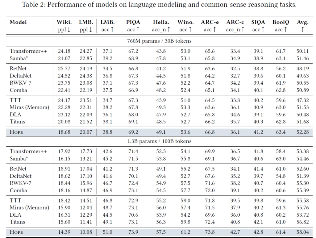
Next, the paper evaluates performance on language modeling and common-sense reasoning tasks. Across these benchmarks, Hope achieves the best average performance compared to all baselines, shown in the right column, both at 760 million and 1.3 billion parameters.
This shows that the architectural changes introduced by Hope do not come at the cost of general language ability.
Continual Learning
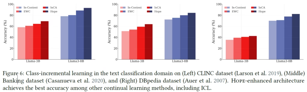
Finally, one of the central goals of the paper is improving continual learning. In the following figure, we can see that Hope outperforms existing continual learning approaches across multiple benchmarks.
References & Links
- Paper page
- Join our newsletter to receive concise 1-minute read summaries for the papers we review – Newsletter
All credit for the research goes to the researchers who wrote the paper we covered in this post.