In this post, we break down Meta AI’s DINOv3 research paper, the latest in their open-source family of computer vision foundation models, now achieving state-of-the-art results with a frozen backbone on many benchmarks.
Introduction
Just as we have large language models (LLMs) serving as general-purpose foundation models for natural language processing (NLP), computer vision is following a similar path with foundation models that can be reused across many tasks. One of the most widely adopted in the past two years has been Meta AI’s DINOv2, which has become one of the go-to backbones in the community.
Now, Meta AI has released the next step in this family: DINOv3. Much like what we’ve seen with LLMs, DINOv3 is both larger and trained on more data, expanding from 1 billion to 7 billion parameters, and from 142 million images to 1.7 billion images.
More parameters, more data. But scaling to this level also introduces new challenges, and some fascinating solutions, which we’ll explore in this post. Specifically, at the end we’ll dive into one of the key innovations that makes DINOv3 work – a method called Gram Anchoring.
But first, let’s quickly revisit what it means to call a model a foundation model in computer vision.
What Are Foundation Models in Computer Vision?
Life Before The Era Of Foundation Models
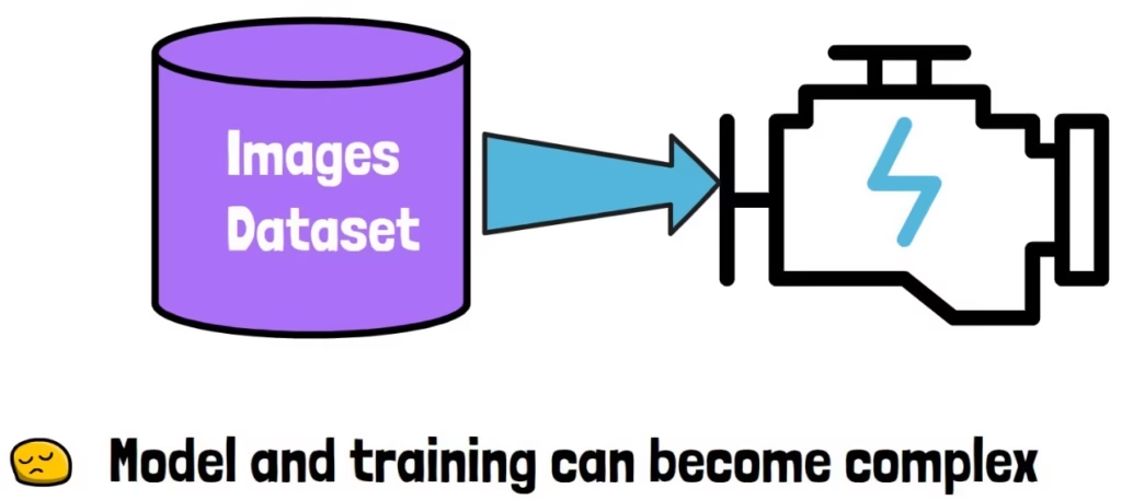
Before the rise of foundation models, building a computer vision system often meant starting from scratch, which involves:
- Collecting or curating a dataset.
- Choosing an architecture.
- Training a model specifically for that task.
This process could be both time-consuming and computationally expensive, especially for complex applications.
DINOv2 changed that. It is a pretrained, large-scale Vision Transformer (ViT) that showed you don’t necessarily need to design or train a specialized, complex model for every new problem. Instead, you could rely on a single general-purpose backbone, and DINOv3 takes this idea to a new level.
Life With A Foundation Model
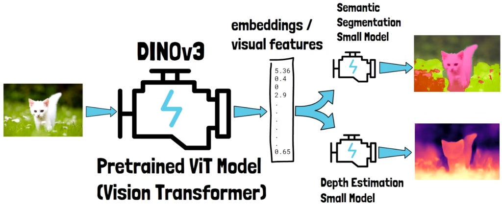
Let’s take a look at a cat image for example (left on the image above). If we pass it through DINOv3, the model produces a vector of numbers, often called embeddings or visual features. These embeddings capture rich information about the image’s content.
Once extracted, you can feed them into smaller, simpler models designed for specific tasks. For instance, one model could perform semantic segmentation, labeling different parts of the image, while another could estimate depth information.
Training Task-Specific Models With DINOv3
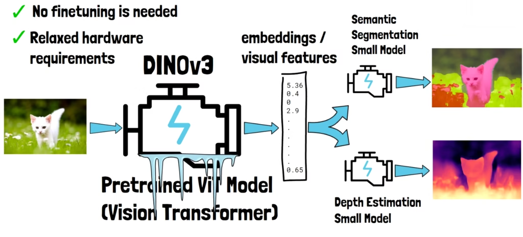
A crucial property of DINOv3 is that it can remain frozen while training these task specific models. In other words, no fine-tuning is required. This makes downstream training much simpler, since DINOv3 processes the image once, and its embeddings can then be reused across multiple task-specific models. This was already true for DINOv2 but now with DINOv3 this approach reaches state-of-the-art results for many tasks.
By contrast, if you fine-tuned the backbone, you’d need to run a separate fine-tuned version for each task, which is costly and impractical. Fine-tuning such a massive model also requires substantial hardware resources, putting it out of reach for many.
DINOv3 Results
Benchmarks Comparison
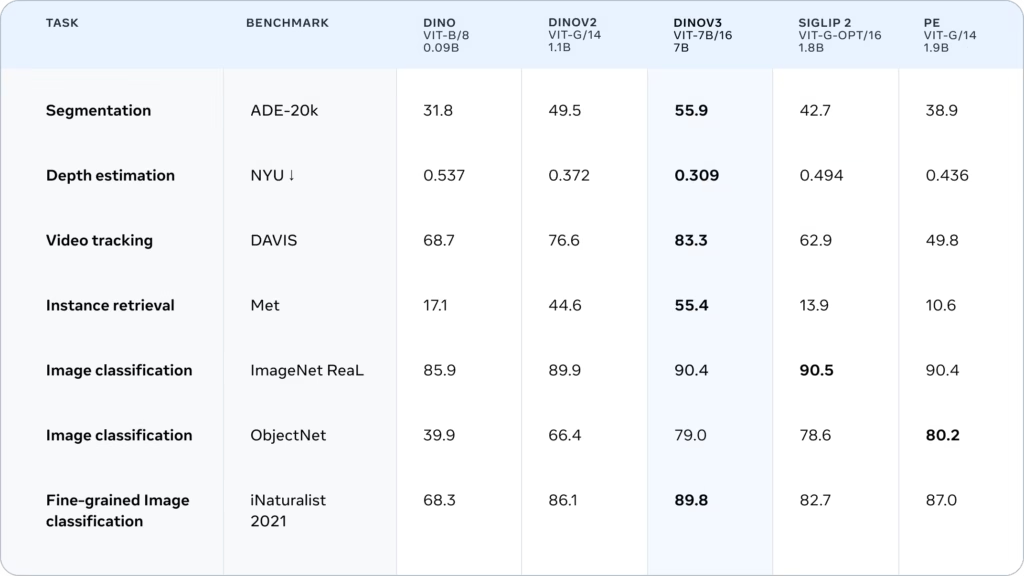
To understand the quality of DINOv3, let’s look at its performance across a wide range of downstream tasks. In the above table, each row represents a specific vision task, and the models compared were trained using frozen embeddings from different backbones. As you can see in the middle column, DINOv3 consistently outperforms DINOv2, as well as Google’s SIGLIP 2 and Meta’s own Perception Encoder, across most tasks.
DINOv3 Features Quality Analysis

To get a feeling of DINOv3’s quality, let’s also take a quick look at the above figure from the paper. In the center, we see a high-resolution image of a fruit stand at a market. Around it, we see similarity maps that were obtained using DINOv3 output, showing how similar are different patches of the image to the patch marked with a red cross in each image.
For example, on the top left, when the red cross is placed on a banana, the similarity map highlights all other banana patches while other patches aren’t. Another example, on the bottom, right where the red cross is placed on a fig, the map shows high-similarity to other fig patches. Actually, on a first look I wasn’t sure why DINOv3 did not show high-similarity for the patches to the left, but then I zoomed in and noticed that it is indeed a different fruit.
Data Curation For Self-Supervised Learning
Let’s now start to understand how DINOv3 was created, beginning with its data curation for training. First, what is self-supervised learning (SSL)? In short, it means we don’t need labels for the training data. The model learns directly from the images themselves, which in principle makes it much easier to scale up.
However, simply scaling up uncurated data has historically hurt performance. DINOv2 already showed that carefully curated, high-quality data works much better.
For DINOv3, the researchers curated three different datasets.
1. LVD-1689M: Curated From Instagram
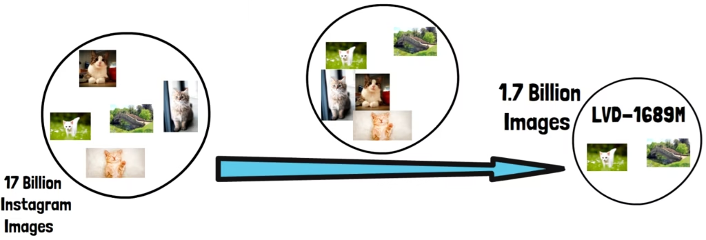
They begin with a massive pool of 17 billion Instagram images and extract 1.7 billion images out of it. This dataset is called LVD-1689M.
- The images were selected by clustering DINOv2 embeddings to ensure balanced coverage across domains.
- This is important since in the original uncurated dataset, we’ll likely find unbalanced bias toward specific domains. For example, it may include a lot of cat images compared to non-cat images.
- Training on such data may lead to a model that is very good in understanding cats but may not do very good in generalizing to other domains.
- By clustering, we basically group the images based on similarities. Afterwards, we can choose from each group a similar number of images to create a more balanced dataset.
2. Task-Specific Expansion
For the second dataset, the researchers take a seed set of images that are particularly useful for specific downstream tasks, and expand it with similar images from the Instagram pool.
3. Publicly Available Datasets
The third part is based on publicly available datasets such as:
- ImageNet1K
- ImageNet22K
- Mapillary Street-level Sequences
Data Selection During Training
During training, these sources are mixed:
- 10% of all batches are homogeneous and include only ImageNet1K samples.
- All other batches randomly mix data from all datasets.
DINOv3 Training Process
Now that we’ve explored DINOv3’s data curation, let’s move on to its training process. DINOv3 combines multiple types of losses, each serving a distinct purpose. Two of these losses, DINO and iBOT, were already present in DINOv2 and complement each other: one captures the global meaning of an image, while the other focuses on local details.
We’ll first break down DINO and iBOT losses, then explain why there are not enough, and how Gram Anchoring solves the problem.
DINO Loss: Capturing Global Understanding
The DINO loss is an image-level loss that helps the model build a consistent global understanding.
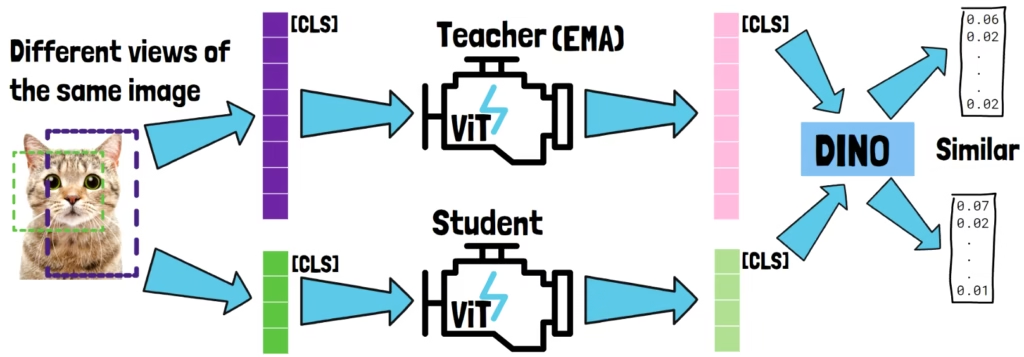
Student And Teacher ViTs Process Different Crops Of The Same Image
Given an input image, we first extract from it a large crop, called a global crop (purple in the image above). That crop is split into a patch tokens sequence which passes via a Vision Transformer (ViT) that generate patch token embeddings. This ViT is the teacher.
Next, we extract another, different, crop, either another global crop of the same size, or a smaller size crop called a local crop. But for the example let’s take a local crop (green in the image above). That second crop is also converted into a patch token sequence. It has less patch tokens since it is smaller and the patch size is fixed. Then, it passes via another Vision Transformer to generate patch token embeddings. The second Vision Transformer is the student.
Explaining The Idea Of The DINO Loss
The input patch token sequences include a learnable class token, noted as [CLS]. The output embeddings for these tokens capture the essence of the entire image. They are passed via a small DINO head that produces a probability distribution over classes. The DINO loss then makes sure that the distributions from the teacher and the student are similar.
So, we feed the teacher and the student models with different views of the same image, and then we verify that the model outputs capture a similar global meaning. This forces the student to actually learn the underlying content of the image, rather than just memorizing the teacher’s outputs.
Self-Distillation: Who Is The Teacher?
The teacher model isn’t trained separately. It is an exponential moving average of the student’s weights across the training iterations. This is a self-distillation process. In fact, the name DINO stands for self-distillation with no labels, to capture this kind of teacher-student self-supervised learning.
The weights average moves slower than the actual student model which contributes to training stability. It also helps to avoid model collapse into a trivial solution.
Multi-Crop Strategy
Meta doesn’t use just two crops as in our example.
- Meta uses two global crops, and eight local crops for each image.
- The teacher processes only the global crops, while the student processes all.
- The loss is applied for each teacher-student pair of non-identical crops.
iBOT Loss: Zooming into Local Details
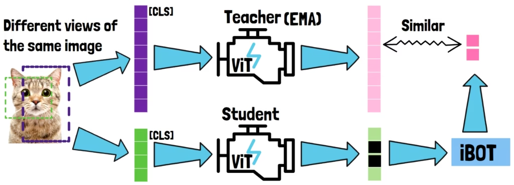
If the DINO loss helps the model to capture the big picture, iBOT helps it zoom into the details. This is a patch-level loss which captures local details, which is especially useful for dense prediction tasks such as segmentation.
Like before, we use the multi-crop strategy. The teacher sees only the global crops, while the student sees both global and local crops.
Explaining The Idea Of The iBOT Loss
Unlike DINOO which compares class-level outputs, this time we focus on the patch tokens. We randomly mask some of the student’s output patch tokens. Then, we pass the masked sequence via an iBOT head, which tries to predict the missing tokens. However, it doesn’t predict the missing student tokens. Instead, it tries to predict the teacher’s output tokens corresponding to the same image location. Then, we verify that the selected teacher output tokens are similar to their prediction from the iBOT head.
The loss is only applied where the student’s masked patches overlap with the teacher’s patches, so there’s enough common ground to compare. For this reason, we take teacher tokens that have sufficient overlap with the student’s crop, and these are the ones being randomly masked.
Another important note is that this is a latent reconstruction objective. Meaning that we reconstruct the latent representations from the teacher network, rather than the original pixels. This encourages the student to learn more semantic features rather than just low-level pixel details.
Shared Computation
iBOT and DINO losses are combined during training, sharing Vision Transformer computations.
Challenges With Scaling DINOv2 To 7B Params
When researchers tried scaling up DINOv2 from 1 billion to 7 billion parameters, the results looked promising on global tasks like classification. But things didn’t go so well for dense prediction tasks such as segmentation.
Global and Local Tasks Performance With Extended Training
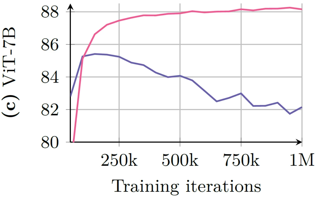
When scaling up the model size and training data, we usually also want to run training for longer. However, in the above figure, we see what happens as training is extended.
- The pink curve shows classification accuracy, which improves over time. As this requires global understanding, we can learn that global understanding gets better with longer training.
- The blue curve shows segmentation performance, which requires strong patch-level understanding. Here, we see a performance drop after a certain point and then stay unstable for the rest of the training.
Visualizing The Dense Features Degradation
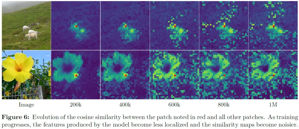
To get some intuition for this, let’s look at the above figure. On the left, we see two images. One with three sheep, and another close-up of a flower. On the right, we see similarity maps at different training checkpoints. These show how the output features relate to the patch marked with a red dot.
At 200k iterations, the similarity maps look smooth and well-localized, meaning the model has consistent patch-level understanding. But by 600k iterations and beyond, things start to fall apart. We see more and more irrelevant patches showing high similarity to the reference patch.
This loss of patch-level consistency correlates with the drop in dense task performance. And this is the motivation for a key innovation in DINOv3, called Gram Anchoring.
Gram Anchoring: Fixing Dense Features
Gram anchoring is another component added to the loss on top of the others we’ve seen. Its goal is to prevent the degradation of patch-level consistency. It is designed to regularize the patch features and ensure a good patch-level consistency, while preserving high global performance.
How Gram Anchoring Works?
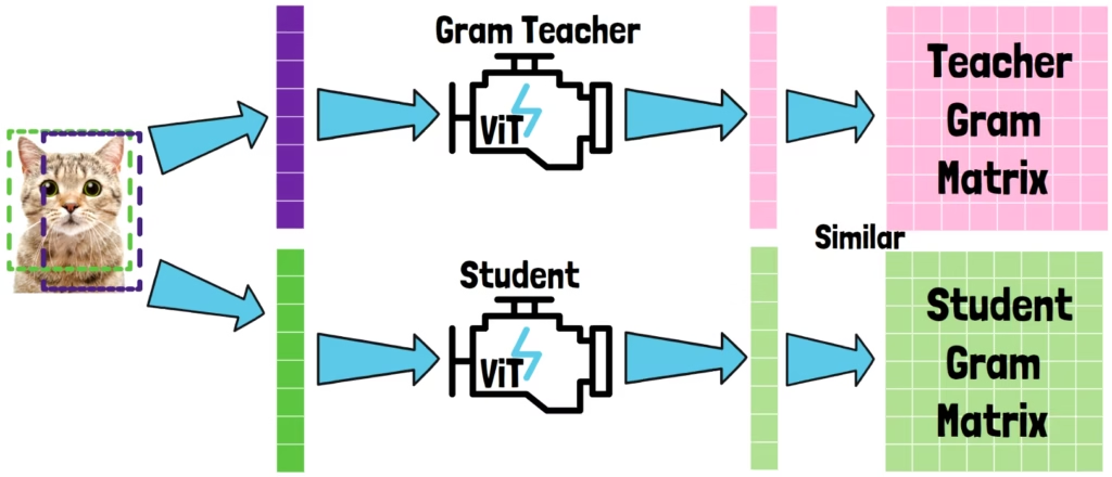
Given an input image, we extract global crops from the image. In this case we only use global crops and not local ones. The crop is converted into a patch sequence, which is processed by the student model to generate patch features. From these patch features, we build a matrix called the Gram matrix.
What Is The Gram Matrix?
The Gram matrix is simply the matrix of all pairwise dot products between patch features. This matrix captures the relationships and similarities between the patch features.
The Gram Teacher
The idea of Gram anchoring is that we take a Gram teacher model which is different than the teacher we used before for DINO and iBOT. The Gram teacher is an earlier checkpoint of the teacher model that we know it has strong dense-tasks performance.
The Gram teacher also processes a global crop of the image to generate its own patch features. Then, we calculate the Gram matrix for the teacher’s output as well.
The Idea Of The Gram Anchoring Loss
The Gram Anchoring loss pushes the student’s Gram matrix to match the teacher’s matrix.
This way we enforce the relationships between the features to remain consistent with that of the Gram teacher. The key is that by operating on the Gram matrix rather than the feature themselves, the features are free to move, as long as the overall structure of similarities remains the same.
Gram Anchoring Performance Boost
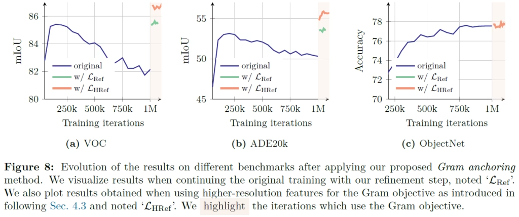
In the above figure from the paper, we can see the impact of Gram Anchoring. Gram Anchoring is only applied after one million iterations, and the results are very impressive.
- On the left and in the middle, we see segmentation benchmarks. Without Gram Anchoring, performance degrades over time. But once it’s added, performance not only recovers but actually surpasses the model’s best earlier results.
- On the right, we see a classification benchmark. Here, global understanding remains strong, showing that Gram Anchoring preserves global performance while stabilizing local features.
A Final Look At DINOv3’s Quality
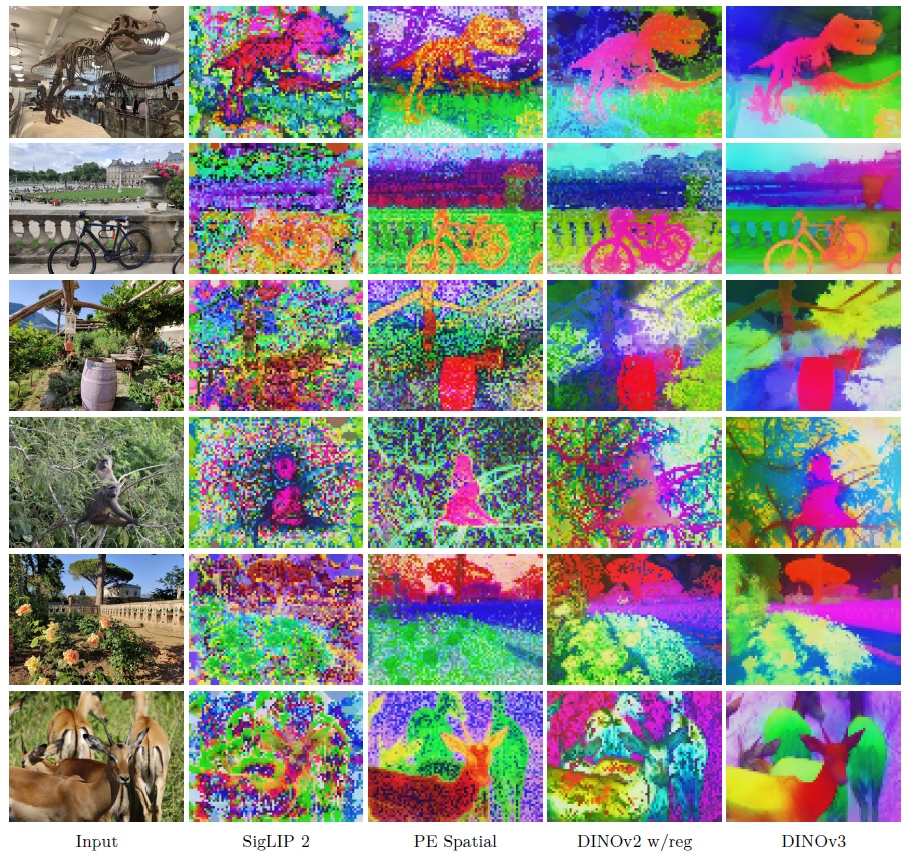
To wrap up, let’s look at one more visualization from the paper. Here we compare dense features of DINOv3, shown on the right, against other top computer vision models. These images are visualized using PCA on the features and mapping to RGB. The DINOv3 features stand out as beautiful and clean, far better than the others.
References & Links
- Paper
- Model
- Join our newsletter to receive concise 1-minute read summaries for the papers we review – Newsletter
All credit for the research goes to the researchers who wrote the paper we covered in this post.