In this post, we dive into a novel AI architecture by sakana.ai called Continuous Thought Machines (CTMs), introduced in a recent research paper of the same name.
Introduction
What if taking AI to the next level means doing something radically different?
The AI architectures that are commonly used today are inspired by the biological structure of the human brain. However, various concepts are intentionally simplified or ignored for the sake of computational efficiency and simplicity. One major simplification is ignoring the concept of time. As humans, we build our thoughts gradually. We reflect, refine and sometimes rethink. But most neural networks respond almost instantly.
Large language models simulate this kind of gradual thinking through long chain-of-thought reasoning processes, which allow them to keep thinking over multiple steps.
CTMs aim to make time a first-class citizen in artificial intelligence, bringing machines a step closer to how our brains actually process the world, while keeping things efficient and relatively simple.
Interestingly, one of the authors, Llion Jones, is also a co-author of the Attention Is All You Need paper, which introduced the Transformer architecture that powers today’s large language models.
Continuous Thought Machines High-Level Architecture
We now describe the various CTM components and its flow. The following drawing is a reference for the upcoming sections.
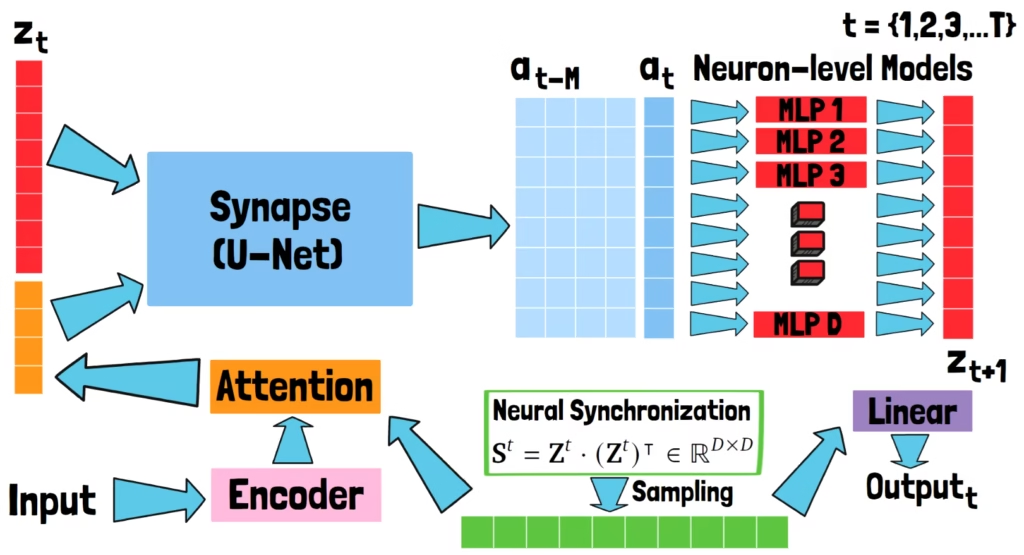
Pre-trained Encoder
To process data, Continuous Thought Machines (CTMs) use an external encoder. The encoder is a pre-trained component, external to the CTM, that transforms raw input into a set of features that the model can operate on.
Internal Time Dimension
The CTM is a recurrent model, but unlike typical recurrent models, where the recurrence is driven by the sequential processing of an input sequence, here the recurrence is controlled by an internal time dimension that is decoupled from the input data. This internal time axis allows the model to unfold its “thoughts” gradually, from step 1 to T. Each of these steps is called an internal tick.
The Synapse
The first trainable component of the Continuous Thought Machine is called the synapse. The researchers experimented with several options for this, and ultimately chose a U-Net architecture for this part.
Now, let’s assume the model has already processed a few internal ticks, and we’re now looking at internal tick t. The input to the U-Net synapse is a combination of the encoded input features and the output from the previous internal tick, denoted with zt.
The synapse processes these together to produce an output called pre-activations, denoted with at.
The Neuron-Level Models
The synapse’s output, the pre-activations are passed to the next major component, the neuron-level models. These are small MLP models, one for each entry in the latent space vector, so D in total, where D is the dimension of the model latent space.
The notion of neuron here is a new abstraction for neurons, unlike the one we know from standard neural networks. This should empower the Continuous Thought Machine to capture complex temporal dynamics.
We have one neuron-level model for each entry in the pre-activations. However, the neuron level models do not process just the current pre-activations. Instead, each one processes a history of pre-activations from previous internal ticks. The size of this history is denoted by capital M, and the paper suggests that values between 10 and 100 work well.
Each neuron-level model processes the history of values for its corresponding dimension in the pre-activations history, and outputs a single value, forming a new vector called the post-activations, denoted by zt+1. The post-activations are fed back into the model as input in the next internal tick.
The idea is that each neuron-level model can decide whether the neuron should be activated or not based on its activation history, using a complex function modeled by an MLP, rather than a static function such as ReLU, allowing the model to capture complex, time-dependent patterns.
So, the synapse captures cross-neuron interactions, and the neuron-level models capture temporal dynamics.
Neural Synchronization
The next component is called Neural Synchronization. This component determines how the Continuous Thought Machine interacts with the world, meaning how it handles inputs and produces outputs.
For each internal tick, the synchronization is represented by a matrix St. In the following equation, we see the synchronization matrix is calculated by multiplying Zt with its own transpose.
An important note is that Zt here is not just the most recent post-activations vector. Instead, it is a matrix containing the post-activations from all previous internal ticks. This way, the neural synchronization captures the ongoing temporal dynamics of neuron activities rather than a single moment snapshot. Each cell (𝑖, 𝑗) in matrix St reflects the synchronization between neurons 𝑖 and 𝑗 over time.
The shape of this matrix is D by D, meaning it depends only on the model’s latent space size and not on the number of previous internal ticks.
However, we don’t use the entire matrix. Instead, we randomly sample a subset of cells from it to form another vector which is referred to as the latent representation of the model.
So, what do we actually do with this latent representation?
The Roles Of The Latent Representation
First, let’s clarify something from earlier. The input data is not fed directly into the synapse component. Instead, it first goes through an attention block. This is where the first role of the latent representation comes in, as another input to the attention block.
The output of this attention block is then concatenated with the latest post-activations vector, and together they form the input to the synapse for the next internal tick.
The second role of the latent representation is generating the model’s output. The latent representation is passed through a linear projection layer to produce the model’s output at internal tick t.
Neural Synchronization – Adding Decay Factor
Let’s revisit the post-activations matrix Zt. It includes the post-activations from all previous internal ticks. But to allow activations from recent internal ticks to have higher impact, the actual formula for the synchronization matrix is actually a bit more complex than just Zt multiplied by its transpose. It also includes a learnable decaying factor which helps the model to scale signals based on their timings.
The First Internal Ticks
An open question you may have by this point is what happens during the early internal ticks, when there’s little or no activation history? The answer is that both z1, the post-activation vector at the first internal tick, and the initial pre-activation history are learnable parameters.
Determining The CTM’s Final Output
As we mentioned earlier, the model generates an output at every internal tick. But how are all of these intermediate outputs are combined together? The answer for this is that it depends on the task.
In the experiments conducted by the researchers, different strategies worked well for different tasks. The different strategies include an average of all the outputs across all internal ticks, or using a single output, either from the last internal tick, or from the tick where the model’s felt most confident.
Confidence, or certainty, is measured using entropy. So for a sequence of outputs, we can compute entropy at each internal tick and pick the one with the highest certainty.
Continuous Thought Machines And Adaptive Compute
The concept of certainty also enables another feature of Continuous Thought Machines, which is adaptive compute. At inference time, the model doesn’t need to run for a fixed number of internal ticks. Instead, it can decide when to stop, based on how confident it is in its output.
This is powerful as it allows the model to finish quickly for simple inputs, but devote more thinking time for complex inputs that require a long reasoning process. This capability is naturally developed during the training process due to how certainty is used as part of training.
Continuous Thought Machines Training Note
During training, the model runs for a full sequence of internal ticks. The loss is then averaged over two specific internal ticks. One is the internal tick where the model had the lowest loss, and the second is the one where the model had the highest certainty. This teaches the model not only how to produce good answers, but also to decide when it’s confident enough to stop thinking.
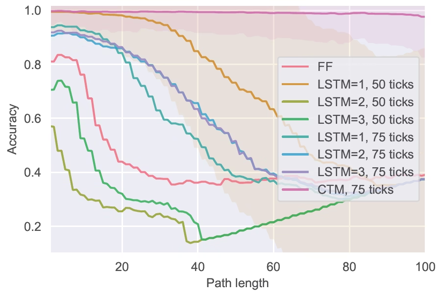
Results Example – 2D Mazes
To see if the architecture actually works, the researchers tested it on a variety of tasks. However, it hasn’t yet been evaluated at a very large scale. Time will tell whether this architecture becomes dominant or not.
We don’t dive into most of the results in this post, but we look into 2D mazes as an example. The model was trained to solve mazes of size 39 by 39, with paths up to 100 steps long. The following figure shows examples for how the Continuous Thought Machine generalizes to longer paths and larger mazes than it saw on training.
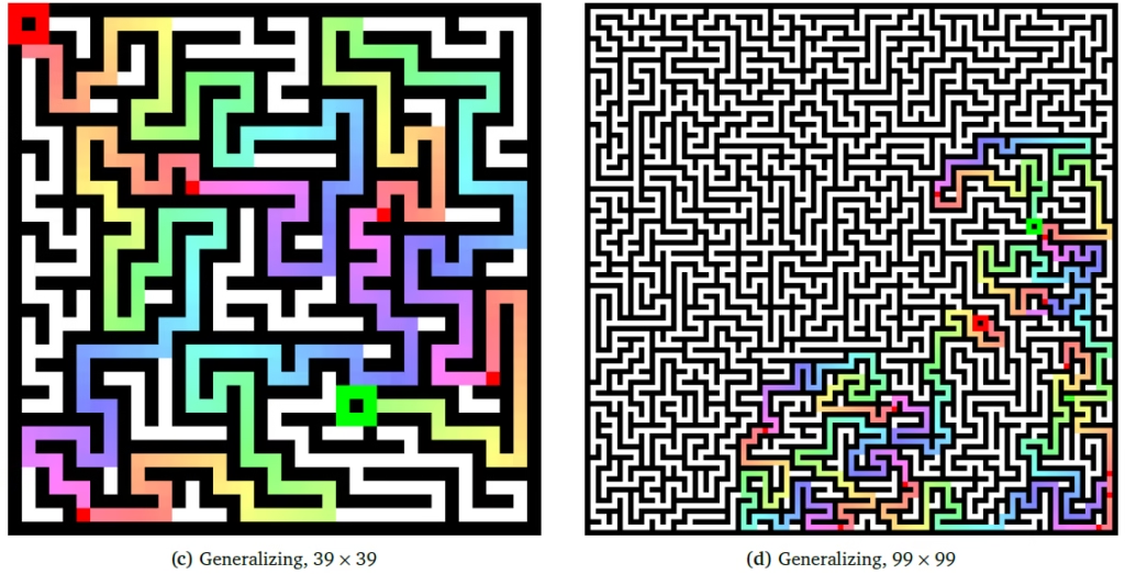
On the left, we see an example for a maze of similar size as in training, but with a longer path. Since the model was trained to generate paths up to 100 steps long, it is being re-applied repeatedly, each time advancing the solution until the full path is complete. The different colors show these successive applications of the model.
On the right we see an example where the model solves a maze of size 99 by 99, much larger than the size encountered in training.
Below, we see a comparison between the CTM and baseline recurrent models which are different versions of LSTM. While some LSTM models are able to solve short-path mazes, only the Continuous Thought Machine consistently solves longer mazes.
References & Links
- Paper Page
- GitHub Page
- Join our newsletter to receive concise 1-minute read summaries for the papers we review – Newsletter
All credit for the research goes to the researchers who wrote the paper we covered in this post.