Introduction

There is no doubt that large language models (LLMs) nowadays are incredibly powerful, possessing extensive knowledge in almost any domain. At the core of these models lies the Transformer architecture. However, to process our prompts, LLMs come with another component before the Transformer, called a tokenizer. The tokenizer converts text into tokens, which are part of the vocabulary of the LLM.
Since the tokens are provided by an external component, the model cannot decide whether to allocate more compute to a certain token, meaning that all tokens are treated the same. However, some tokens are much harder to predict than others. For example, the first token in a sentence is harder to predict compared to the ending of most words. Additionally, this leads to other shortcomings, such as a lack of orthographic knowledge, which is the understanding of the spelling system and its patterns.
In this post, we dive into a recent paper by Meta, titled: “Byte Latent Transformer: Patches Scale Better Than Tokens.” The paper introduces the Byte Latent Transformer, or BLT for short, a tokenizer-free architecture that learns from raw byte data. Processing the sequence byte by byte results in very large sequences, which in turn creates scaling issues for byte-level models. To mitigate this, the Byte Latent Transformer dynamically groups bytes into patches and performs most of its processing on these patches. Let’s explain how it works.

Strategies to Divide the Byte Sequence into Patches
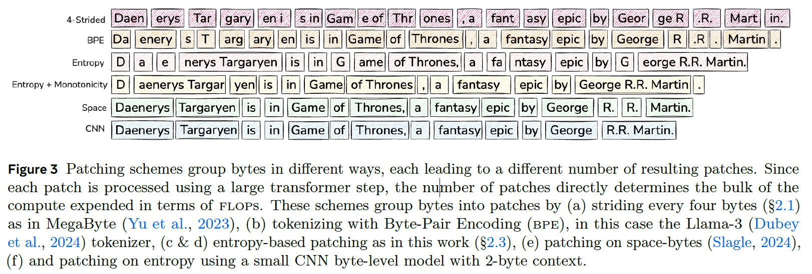
Let’s start by reviewing several strategies to divide the byte sequence into patches, using the following figure from the paper. In this figure, we have a sentence for example: “Daenerys Targaryen is in Game of Thrones, a fantasy epic by George R.R. Martin.” and we see how each strategy would group the bytes into patches.

4-Strided Approach
In the first approach, called 4-Strided, we create patches of a fixed size of 4 bytes. This means we create a patch for every 4 bytes. While this approach is beneficial due to its simplicity, it does not dynamically allocate compute where it is needed the most. Additionally, similar byte sequences may suffer from inconsistent patching, as we could split the same word in different locations, depending on where it is located in the sentence.
Byte-Pair Encoding (BPE)
BPE stands for Byte-Pair Encoding, which is a subword tokenization used in many large language models, such as LLaMA 3. This approach is commonly seen in current LLMs.
Space Patching
In this simple approach, we start a new patch after any space-like byte. One advantage here is that we have consistent patching, since we will patch the same word in the same way in any sequence. Additionally, predicting the beginning of a word is usually more challenging than predicting the rest of the word, and in this way, we ensure that compute is allocated for every word. However, this method does not fit all languages and domains, such as math. Additionally, this mechanism cannot vary patch size, as it is determined by the word’s length.
Entropy-based Patching
Entropy patching provides a dynamic allocation of compute where it is needed the most. Entropy is a measure of uncertainty. High entropy means high uncertainty, while low entropy means low uncertainty. The entropy here is calculated over the prediction of the next byte using a small byte-level language model trained for this purpose. If the small byte-level language model has high uncertainty for predicting the next token, it can be a good hint that the next byte is a hard one to predict.

In the above figure from the paper, we can see how the patches are constructed for the example sentence. The x-axis shows the bytes for the example sentence, and the y-axis presents the entropy of predicting the next byte. The red dotted line is the threshold to determine whether a new patch should be started. we see at the beginning that there is high entropy for predicting each of the first bytes, which results in a patch for each of the first three bytes. Afterwards, when we already have the prefix “D-a-e”, it is more likely that we will complete to “Daenerys Targaryen,” and so there is lower entropy until the end of the word “Targaryen”, which results in a longer patch, and so it goes to build the patches for the entire sequence.
Entropy + Monotonicity

This method can be understood using the above equations. The upper one represents the entropy method, setting a threshold for the entropy for predicting the next byte. The lower one represents the Entropy + Monotonicity method, where the criteria for creating a new patch is not the entropy value, but rather the difference between the entropy of predicting the next byte and the entropy for predicting the current byte.
CNN Approach
The Convolutional Neural Network (CNN) patching method is also based on entropy, but instead of a small language model, it uses a CNN.
Byte Latent Transformer (BLT) Architecture
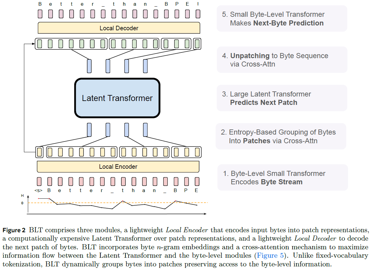
Let’s now review the high-level architecture of the Byte Latent Transformer model. We will use the following figure from the paper. The architecture comprises three key modules: the Local Encoder, the Latent Transformer, and the Local Decoder.

Local Encoder
We start at the bottom with the Local Encoder. Its inputs are embeddings of a byte sequence. Each byte embedding is a combination of multiple n-gram embeddings, providing context about the preceding bytes. The Local Encoder encodes the input byte embeddings using a lightweight byte-level Transformer. Additionally, it is responsible for creating the patch sequence. The grouping of bytes into patches is based on the entropy method we covered earlier. We can see the next byte prediction entropy at the bottom. We’ll expand on the creation of the patch sequence soon, but for now, note that it is done using cross-attention between the byte sequence and an initial patch sequence.
Latent Transformer
Next, the patch sequence is the input to the Latent Transformer, which is the main and large component of the Byte Latent Transformer. It processes the patches to provide output patch representations.
Local Decoder
Finally, we have the Local Decoder. We’ll expand on the Local Decoder soon, but at a high level, it unpatches the output from the Latent Transformer to a byte sequence via cross-attention with the output of the Local Encoder, provided using a residual connection that bypasses the Latent Transformer. The Local Decoder comprises another small byte-level Transformer, which is used to predict the next byte.
Diving Deeper into the Local Encoder and Local Decoder
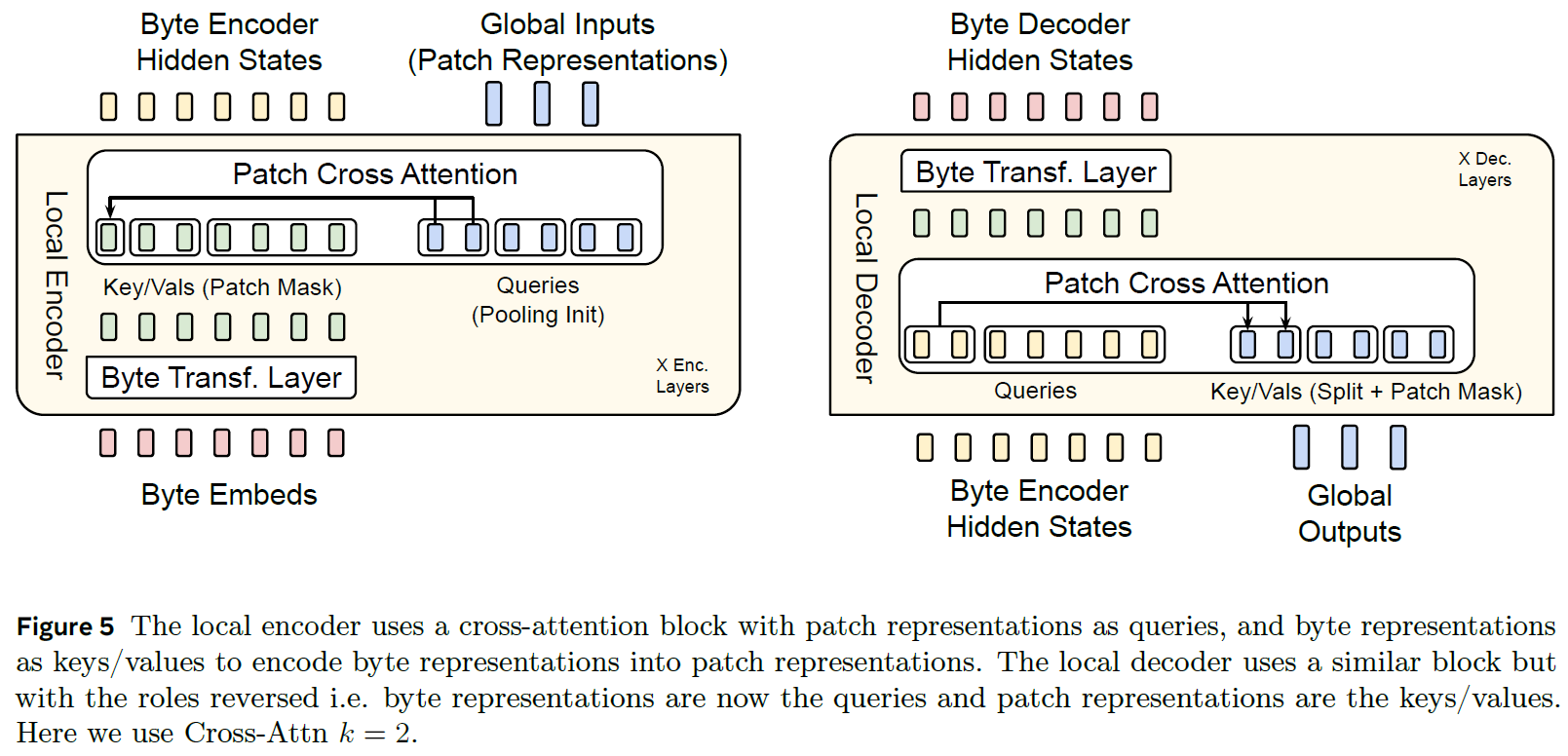
To understand better, we now dive deeper into the Local Encoder and the Local Decoder, using the following figure from the paper.

Inner Architecture of the Local Encode
On the left of the above figure, we see the inner architecture of the Local Encoder. Its inputs are the byte embeddings, and it also starts with an initial patch sequence representation. The figure mentions it is done using pooling init, meaning that the initial representation of the patches is constructed as a combination of the relevant byte embeddings for each patch, converted to the dimensions of the patch. Here, each patch gets two vectors for its representation, determined by a hyperparameter k.
The byte embeddings are first passed via a Transformer layer, where the self-attention is masked so each byte will attend only a window of preceding bytes. The output of the Transformer layer is then used as the keys and values in a cross-attention block, where the patches are used as the queries. Masks are used so each patch will only attend byte embeddings in its scope, though recall that the byte embeddings can have context from previous patches thanks to the n-gram embeddings and the byte-level Transformer layer.
The output of the cross-attention block is the patch representation’s hidden states, which distills information from the relevant bytes for each patch. Multiple layers of the Local Encoder are stacked, each providing the encoded bytes and the patch representations as output for the next layer.
Inner Architecture of the Local Decoder
On the right of the above figure we see the inner architecture of the Local Decoder. It receives the encoded bytes from the Local Encoder and the patch outputs from the Latent Transformer. The Local Decoder is essentially an inversion of the Local Encoder.
It starts with a cross-attention block to unpatch the output patches into a byte sequence. The roles in the cross-attention block are now switched compared to the Local Encoder. The patches are used as keys and values, while the byte encoder hidden states are used as the queries. The cross-attention retains the dimensions of the queries, resulting in a byte sequence enriched with information from the patches. Next, this enriched byte sequence passes via a byte-level Transformer layer, generating hidden states.
The Local Decoder layers are stacked, with each layer receiving the byte decoder hidden states from the previous layer, and the same output patches from the Latent Transformer
Byte Latent Transformer Results
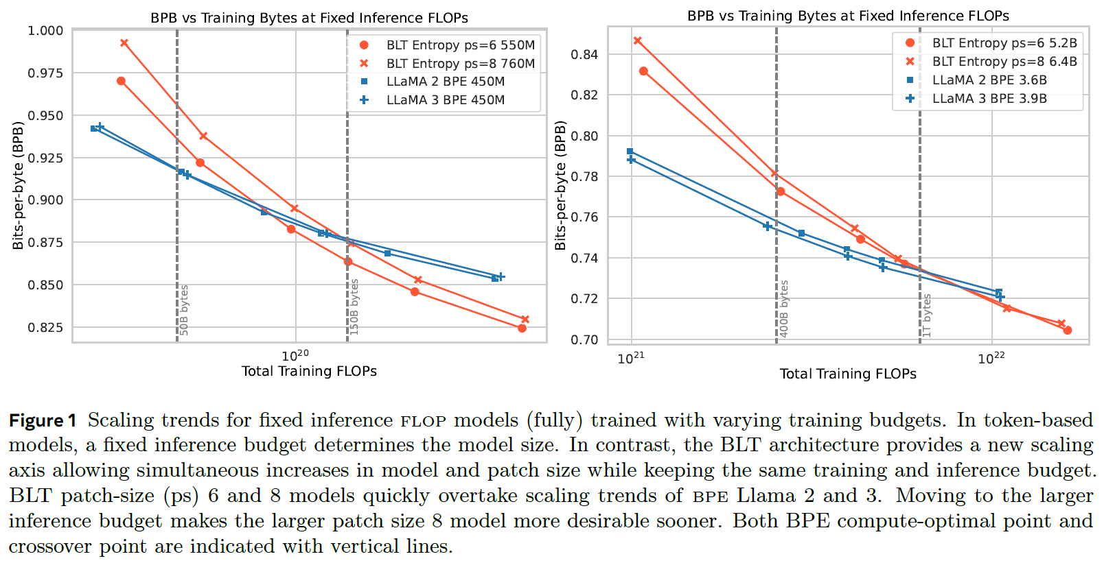
In this section, we review some of the results presented in the paper, using the following figure.

Understanding the Metrics
Both charts below have the training budget on the x-axis and the bits-per-byte (BPB) metric on the y-axis. The bits-per-byte metric measures the average number of bits required to predict the next token in a sequence, which is usually a byte. A lower bits-per-byte value indicates that the model requires fewer bits to predict the next token, thus making it more efficient.
Small Model Comparison
On the left, we see the results for smaller models. The blue lines represent LLaMA 2 and LLaMA 3 models with 450 million parameters, which use standard byte-pair encoding tokenization. The orange lines represent the Byte Latent Transformer models with patch sizes of 6 and 8, which have a larger number of parameters than the LLaMA models. Despite the larger size of the Byte Latent Transformer models, the evaluation is conducted using the same training budget. It is evident that at a certain point, the Byte Latent Transformer surpasses the LLaMA models in terms of efficiency and performance.
Large Model Evaluation
On the right, we observe the evaluation results for larger models. Here, the Byte Latent Transformer models are again trained using the same training budget as the smaller LLaMA models. The results show that with sufficient training, the larger Byte Latent Transformer models achieve better bits-per-byte results, highlighting their superior efficiency and performance compared to the traditional LLaMA models.
References & Links
- Paper
- Code
- Video
- Join our newsletter to receive concise 1-minute read summaries for the papers we review – Newsletter
All credit for the research goes to the researchers who wrote the paper we covered in this post.